

Form 8-K PROGRESSIVE CORP/OH/ For: Aug 12
 Tweet
Tweet Share
Share
UNITED STATES
SECURITIES AND EXCHANGE COMMISSION
Washington, D.C. 20549
FORM 8-K
CURRENT REPORT
Pursuant to Section 13 or 15(d)
of the Securities Exchange Act of 1934
Date of Report (Date of earliest event reported) August 12, 2016
THE PROGRESSIVE CORPORATION
(Exact name of registrant as specified in its charter)
| Ohio | 1-9518 | 34-0963169 | ||
| (State or other jurisdiction of incorporation) |
(Commission File Number) |
(IRS Employer Identification No.) |
6300 Wilson Mills Road, Mayfield Village, Ohio 44143
(Address of principal executive offices) (Zip Code)
Registrant’s telephone number, including area code 440-461-5000
Not Applicable
(Former name or former address, if changed since last report)
Check the appropriate box below if the Form 8-K filing is intended to simultaneously satisfy the filing obligation of the registrant under any of the following provisions (see General Instruction A.2. below):
| ¨ | Written communications pursuant to Rule 425 under the Securities Act (17 CFR 230.425) |
| ¨ | Soliciting material pursuant to Rule 14a-12 under the Exchange Act (17 CFR 240.14a-12) |
| ¨ | Pre-commencement communications pursuant to Rule 14d-2(b) under the Exchange Act (17 CFR 240.14d-2(b)) |
| ¨ | Pre-commencement communications pursuant to Rule 13e-4(c) under the Exchange Act (17 CFR 240.13e-4(c)) |
Item 7.01 Regulation FD Disclosure.
On August 12, 2016, The Progressive Corporation released a Report on Loss Reserving Practices (the “Report”), which provides a discussion of the loss reserving practices used by Progressive’s insurance subsidiaries. A copy of the Report is attached hereto as Exhibit 99.
Item 9.01 Financial Statements and Exhibits.
| (d) | Exhibits. |
See exhibit index on page 4.
- 2 -
SIGNATURES
Pursuant to the requirements of the Securities Exchange Act of 1934, the Registrant has duly caused this report to be signed on its behalf by the undersigned hereunto duly authorized.
| Dated: August 12, 2016 |
||||||
| THE PROGRESSIVE CORPORATION | ||||||
| By: | /s/ Jeffrey W. Basch |
|||||
| Name: Jeffrey W. Basch |
||||||
| Title: Vice President and Chief Accounting Officer |
||||||
- 3 -
EXHIBIT INDEX
| Exhibit No. | Form 8-K | |||
| Under Reg. | Exhibit | |||
| S-K Item 601 |
No. |
Description | ||
| 99 | 99 | The Progressive Corporation’s Report on Loss Reserving Practices, dated August 2016 | ||
- 4 -
Table of Contents
Exhibit 99

Table of Contents
Preface
The artwork1 on the cover of the 2016 Report on Loss Reserving Practices shows a thread tying together a variety of triangles. The thread is a Progressive-wide symbol that ties together our brand, our people, and our customers. The thread runs through us and binds us toward a common goal. In loss reserving, our goal is to accurately set reserves. We tie together data, often in the form of triangles, to reach this goal. The thread runs through us.
The primary purpose of this report is to help interested stakeholders better understand our loss reserving process and how it affects our financial results. Reserves in this report refer to loss and loss adjustment expense reserves.
The 2016 Report on Loss Reserving Practices is very similar to the 2015 report. However, we updated financial information throughout the report.
As the Appendix is a separate document, you can electronically link to it anywhere that you see the blue underlined word: Appendix.
Consistent with Progressive’s culture of self-examination, our analysis of loss reserves demands continuous change and continuous improvement. Each section of this report focuses on a different aspect of our reserving process.
| ● | Section I provides an overview of our financial objectives and results, and explains why accurate reserving is important |
| ● | Section II defines our overall goal of the reserving process, the different types of reserves, how they are related and how we analyze them |
| ● | Section III defines reserve development and describes how it affects our financial results, and also how historical results compare to our goal of having total reserves that are adequate and develop with minimal variation |
| ● | Section IV describes how and why we estimate our required reserves by segment |
| ● | Section V defines many of the terms we use throughout the report |
| ● | Sections VI and VII in the Appendix present two case studies of segment reserve reviews – one for loss reserves and one for Loss Adjustment Expense (LAE) reserves, including discussion of the issues we consider and the calculations involved |
The 2016 Report on Loss Reserving Practices was revised by Karen VanCleave. Despite the technical nature of our reserve analysis, we strive to make this report as accessible and understandable as possible to a wide audience. We welcome your comments so that we may continue to enhance it. Comments and questions should be directed to Gary Traicoff, Corporate Actuary or Karen VanCleave, Actuarial Director, at The Progressive Corporation, 6300 Wilson Mills Road, Mayfield Village, Ohio 44143 or e-mailed to [email protected] or [email protected].
1 Artwork for the cover of this report was designed by **John Burke.
Table of Contents
Safe Harbor Statement Under the Private Securities Litigation Reform Act of 1995: Investors are cautioned that certain statements in this report not based upon historical fact are forward-looking statements as defined in the Private Securities Litigation Reform Act of 1995. These statements often use words such as “estimate,” “expect,” “intend,” “plan,” “believe,” and other words and terms of similar meaning, or are tied to future periods, in connection with a discussion of future operating or financial performance. Forward-looking statements are based on current expectations and projections about future events, and are subject to certain risks, assumptions and uncertainties that could cause actual events and results to differ materially from those discussed herein. These risks and uncertainties include, without limitation, uncertainties related to estimates, assumptions, and projections generally; inflation and changes in general economic conditions (including changes in interest rates and financial markets); the accuracy and adequacy of our pricing, loss reserving, and claims methodologies; the competitiveness of our pricing and the effectiveness of our initiatives to attract and retain more customers; our ability to obtain regulatory approval for requested rate changes and the timing thereof and for any proposed acquisitions; legislative and regulatory developments at the state and federal levels, including, but not limited to, matters relating to vehicle and homeowners insurance; the outcome of litigation or governmental investigations that may be pending or filed against us; severe weather conditions and other catastrophe events; the effectiveness of our reinsurance programs; changes in driving and residential occupancy patterns; our ability to accurately recognize and appropriately respond in a timely manner to changes in loss frequency and severity trends; technological advances; court decisions, new theories of insurer liability or interpretations of insurance policy provisions and other trends in litigation; changes in health care and auto and property repair costs; and other matters described from time to time in our releases and publications, and in our periodic reports and other documents filed with the United States Securities and Exchange Commission.
Table of Contents
| 1 | ||||
| 1 | ||||
| 1 | ||||
| 2 | ||||
| 3 | ||||
| 6 | ||||
| 7 | ||||
| 7 | ||||
| 10 | ||||
| 11 | ||||
| 12 | ||||
| 12 | ||||
| 14 | ||||
| 14 | ||||
| 15 | ||||
| External Reporting of Reserve Changes and Reserve Development |
17 | |||
| Internal Reporting of Reserve Changes and Reserve Development |
19 | |||
| 20 | ||||
| 21 | ||||
| 24 | ||||
| Appendix | ||||
| Appendix | ||||
| 01P00102.A (07/13) | Copyright © Progressive Casualty Insurance Company. All Rights Reserved. |
Table of Contents
The Progressive insurance organization began business in 1937. The Progressive Corporation, an insurance holding company, was formed in 1965. In April 2015, The Progressive Corporation acquired a majority interest in ARX Holding Corp (“ARX”). The financial results include The Progressive Corporation and ARX and their respective wholly owned insurance and non-insurance subsidiaries and affiliates (references to “subsidiaries” include affiliates as well).
The insurance subsidiaries provide personal and commercial vehicle and property insurance and other specialty property-casualty insurance and related services. Our property-casualty auto insurance products protect our customers against losses due to collision and physical damage to their insured motor vehicles, uninsured and underinsured bodily injury, and liability to others for personal injury or property damage arising out of the use of those vehicles. Our property insurance products protect homeowners, other property owners, and renters against losses caused by fire, windstorms, hail, lightning, theft, or vandalism, among certain other losses. Our non-insurance subsidiaries generally support our insurance and investment operations.
We operate our personal and commercial auto businesses throughout the United States, and sell personal auto physical damage and auto property damage liability insurance in Australia. Our homeowners business is underwritten by select carriers, including ARX, in most states throughout the U.S.
Progressive generated net income of $1.27 billion, or $2.15 per share, for 2015. From an operations standpoint, the Company generated an underwriting profit of 7.5% which exceeded our targeted goal of 4.0%. The Company generated $20.6 billion of net written premiums across all business units, an increase of 10% from the prior year. Policies in force—our preferred measure of growth—increased 3.9% for our vehicle businesses, which represented almost 544,000 additional policies. Our 2015 results show a Return on Shareholders’ Equity (ROE) of 17.2%2 and a Comprehensive ROE of 14.2%3.
Progressive’s vision is to be consumers’ number one choice and destination for auto and other insurance. Our financial objectives balance and prioritize our desire for growth with the desire to maintain financial stability that enables us to have lasting relationships with our customers based on our ability to deliver on the promises we make them.
We measure ourselves against two specific goals designed to maximize the value of our Company. Our most important goal is for our insurance subsidiaries to produce an aggregate
2 Based on net income
3 Use of Comprehensive ROE is consistent with the Company’s policy to manage on a total return basis and reflects changes in unrealized gains and losses on securities held in our portfolio. This is our preferred measure of business profitability and capital efficiency. For Progressive, Comprehensive ROE consists primarily of:
| (Net Income) + (Changes in Unrealized Security Gains, Net of Taxes)
|
||||
|
|
||||
| (Average Shareholders’ Equity) |
To review all components of Progressive’s Comprehensive ROE, refer to our “Consolidated Statements of Comprehensive Income” and related notes in our 2015 Annual Report to Shareholders, which is attached as an appendix to the Company’s 2016 Proxy Statement.
Page 1
Table of Contents
calendar year underwriting profit of at least 4%. Second, we seek to grow our business as fast as possible so long as doing so is consistent with our profitability objective and our ability to provide high quality service. We communicate these two corporate goals to every Progressive employee and work together to achieve them.
Our financial policies evaluate our exposure to risk, including the chance that actual events turn out to be significantly different than expected and result in a loss of capital. Our Risk Management area, along with our business units, identifies risks that have the potential to significantly impair our strategic objectives. We use risk management tools to quantify the amount of capital needed, in addition to surplus, to absorb consequences of unfavorable but foreseeable events. These events include items such as unfavorable loss development, weather catastrophes, and investment market corrections, among other events. We include these estimates in our capital models.
Our risks are classified into the following four categories:
| ● | Insurance Risks – risks associated with assuming, or indemnifying for, the losses of, or liabilities incurred by, policyholders |
| ● | Operating Risks –risks stemming from external or internal events or circumstances that may directly or indirectly affect our insurance operations |
| ● | Market Risks – risks that may cause changes in the value of assets held in our investment portfolios, and |
| ● | Credit and Other Financial Risks – the risks that the other party to a transaction will fail to perform according to the terms of a contract or that we will be unable to satisfy our obligations when due or obtain capital when necessary |
Loss reserving is a source of insurance risk because significant variations in loss reserve estimates affect our operating profit and our ability to price accurately.
Loss reserving is an activity that is central to the achievement of our goals. It involves estimating the magnitude and timing of future claim payments and loss adjustment expenses for accidents that have already occurred. These estimates take into account not only claims that are in the process of being settled but also claims on accidents that have occurred but have not yet been recorded by the Company. The latter is known as Incurred But Not Recorded, or IBNR claims. At year-end 2015, Progressive’s estimated gross Loss and Loss Adjustment Expense (LAE) reserves amounted to $10.0 billion.
Relationship between Loss Reserving and Pricing Functions
Unlike most industries, insurers do not know their costs until well after a sale has been made. Thus, one of the most important functions for an insurance company is setting rates or pricing. The goal of our pricing function is to properly evaluate future risks the Company will assume but has not yet written. Estimates of future claim payments are essential for accurately measuring Progressive’s underwriting profit and for determining whether pricing changes are needed to achieve the Company’s underwriting target. Reserve estimates that are too low can lead to the conclusion that pricing is adequate when it is not, and additionally, we may experience unprofitable growth. Reserve estimates that are too high may lead to inflated prices, potentially limiting our ability to attract and retain customers.
Our product-focused business units continue to seek ways to advance the science of rate-making to achieve accurate cost-based pricing at the most detailed level our data will support. This allows us to more accurately match our rates with expected loss costs by risk classification.
The role of the pricing function is to determine rates that are adequate to achieve our profitability goals without being excessive or unfairly discriminatory to consumers. The Pricing Group develops their own projections of ultimate losses for the purposes of ratemaking. The Loss
Page 2
Table of Contents
Reserving Group’s projections of ultimate loss may also be considered by the Pricing Group when they are generating these projections. Although the pricing function is very different from the loss reserving function, the data used is consistent between the functions. Typical information that the Loss Reserving Group shares with the Pricing Group includes:
| ● | Overall changes in the level of reserves by type of reserve (see Section III) |
| ● | History of claim development and selected ultimate losses by accident period |
| ● | Changes in selected ultimate loss amounts over time |
| ● | Selected severity by historical accident period and resulting trends |
| ● | Selected frequency by historical accident period and resulting trends |
| ● | Changes in actuarially determined case average reserves by age (see Section III) |
| ● | Changes in the level of average adjuster case reserve estimates (see Section III) |
| ● | Changes in claim closure rates |
| ● | Changes in the closed without payment (CWP) rate |
Judgments made by both the Loss Reserving and Pricing Groups consider additional information. Growth and process changes may cause claims to settle faster or slower than previous experience. Changes to regulatory requirements made by state insurance departments, as well as changes in the mix of business and in the underwriting process, may also contribute to unexpected changes in the data.
We use a cost-plus strategy in pricing, beginning with the projected ultimate losses and LAE. The Pricing Group estimates the ultimate losses and LAE for each coverage for the state under review. Their projection methods are similar to those used by the Loss Reserving Group, as described in Section IV.
Trend selections have a significant impact on how much the rates will change. Changes in the average cost of a claim (severity trend), in the proportion of insured cars that have a claim (frequency trend), and in average premium adjusted for current rate levels (premium trend) are analyzed and selected.
The Loss Reserving Group meets regularly with the Product Management Group, Pricing Group and Claims Group to discuss these trends.
Loss Reserve Uncertainty and Capital Planning
With recommended regulatory changes and other developments (Solvency II & Own Risk Solvency Assessment or ORSA), companies taking advantage of Loss Reserve Disclosures are likely to benefit in many ways. Disclosure regarding an insurer’s practice of setting loss reserves, generally an insurer’s largest balance sheet liability, helps explain business decisions to investors, rating agencies and other interested parties such as regulators, employees and other stakeholders in the firm. Disclosures such as this 2016 Report on Loss Reserving Policies, which we file with the SEC on Form 8-K, allow management to explain its rationale and practices in setting reserves, the methods used to model reserves and the varying degree of results that are produced by various reserving methods.
Actuarial estimates of future loss payments resulting from accidents that have already occurred are imprecise by their nature. The amount that will actually be paid is uncertain for many reasons and may deviate, sometimes substantially, from the estimated liability. Because loss reserves are inherently imprecise, insurers are faced with the real risk that they will pay out differently than they have estimated. It is for this reason that Progressive’s Risk Management area built a loss reserve estimation risk model which measures the magnitude of that potential difference between what we forecast to happen and actual loss payments made. We use the results of this model in conjunction with other risk models to determine the amount of Economic Capital held for the consolidated entity.
Page 3
Table of Contents
Economic Capital can be defined as the amount of capital that a business needs to ensure that it remains solvent. Economic Capital is a measure of risk, not of actual capital available to the business. As such, it is distinct from familiar accounting and regulatory capital measures. Economic Capital is based on a probabilistic assessment of potential future losses and is therefore a more forward-looking measure of capital adequacy than traditional accounting measures. Progressive calculates Economic Capital internally as the estimated additional capital we need to withstand potential losses from all sources of risk. Progressive uses the Value at Risk measure, or VaR, which is defined as a threshold loss value, such that the probability that the aggregate losses exceeds a selected confidence level. The VaR measurement process involves assigning to each given risk an amount of capital that would be required to respond to any unexpected loss, while taking account of the diversification benefits of managing a portfolio of risks, some of which are not highly correlated. Volatility in losses results in volatility in estimated loss reserves, which in turn increases the amount of Economic Capital required for capital planning purposes.
Loss reserve uncertainty arises for a variety of reasons. Therefore, no single method of estimating loss reserve uncertainty is appropriate under all circumstances. For example, unanticipated spikes in medical inflation will result in actual loss payments that exceed our estimates (an unanticipated increase in reserve need). By contrast, changes in claims handling procedures may allow us to settle claims more quickly and efficiently than previously thought, with the result of lower actual adjusting expenses than previously estimated (an unanticipated decrease in reserve need). Even different types of hurricanes must be reviewed independently as reserve development from one hurricane can be very different from another. See the graph below.
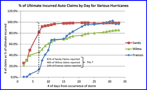
We see in the above graph that three different hurricanes and tropical storms created very different claim reporting patterns within the first seven to ten days. Wilma, a typical hurricane, hit urban areas which caused flooding, but the flood waters retreated fairly quickly allowing policyholders to return home and report damages within a reasonable period of time. Frances, a storm with a large eye that struck during Labor Day weekend, caused significant flooding and resulted in delayed reporting patterns. Superstorm Sandy on the other hand, the second costliest
Page 4
Table of Contents
storm in US history (estimated at $75B USD) with a diameter on record of 1,100 miles, allowed policyholders’ early re-entry into the affected area. Losses were reported quickly, resulting in prompt claim settlements. As you can see in the graph above, by day 15, nearly all of the Superstorm Sandy claims were reported allowing for improved reserve accuracy and less dependency on estimates for incurred but not reported (IBNR) claims.
Modeling loss reserve uncertainty is accomplished by using historical loss payment data to statistically estimate the relationship between loss payments made in the first development year of each accident year and payments in each subsequent development year. Although these statistical relationships are accurate on average, actual loss payments do vary as discussed above. The risk management model measures the magnitude (standard deviation) of these variations as a percentage of the estimated needed reserve and applies this estimate to expected future loss payments.
We currently estimate loss reserve uncertainty separately from loss adjustment expense reserve uncertainty because economics, process, pricing and other changes may affect loss adjustment reserves differently from loss reserves. Unanticipated fluctuations can occur for many reasons some of which include:
| ● | History of claim development and selected ultimate losses by accident period |
| ● | Changes in claim closure rates |
| ● | Selected severity by accident period and resulting trends |
| ● | Selected frequency by accident period and resulting trends |
| ● | Unanticipated spike in medical inflation |
| ● | Changes in the rate of claims closed without payment (CWP rate) |
| ● | Acute change (increase/decrease) in driving behaviors of our policyholders |
| ● | Economic factors such as inflation/deflation |
| ● | Unanticipated changes in the costs of repairing vehicles |
The loss reserve estimation risk model results are combined with other stochastic risk models such as investment portfolio returns, operating risk and other financial risks to determine the total Economic Capital required at various confidence levels.
Page 5
Table of Contents
Section II – Key Definitions and Types of Reserves
In order to understand Progressive’s Reserving Practices, it is important to first have an understanding of our overall goal as well as several definitions of various types of reserves. Additional definitions can be found in our Glossary in Section V.
Reserves are liabilities established on our Generally Accepted Accounting Principles (GAAP) balance sheet as of a specific accounting date. They are estimates of the unpaid portion of what we ultimately expect to pay out on claims for insured events that occurred prior to the end of any given accounting period, regardless of whether or not those claims have been recorded by Progressive. These estimates are reported net of the anticipated amounts recoverable from salvage and subrogation. Loss reserves are our best estimate of future payments to claimants, and LAE reserves are the estimated future expense payments related to claims settlement. The types of reserves are explained below.
We estimate the needed reserves based on facts and circumstances known to us at the time the loss and LAE costs are evaluated. There is inherent uncertainty in the process of establishing property and casualty loss and LAE reserves, caused in part by changes in the Company’s mix of business (by state, policy limit or deductible, etc.), changes in claims staffing and processes, inflation on vehicle repair costs and medical costs, changes in state legal and regulatory environments, and unexpected judicial decisions regarding lawsuits, changes in theories of liability, and interpretation of insurance policy provisions, among other reasons.
|
Progressive’s goal is to ensure that total reserves are adequate to cover all loss and LAE costs while sustaining minimal variation from the time reserves are initially established until losses have fully developed.
|
The Corporate Actuary is accountable for the adequacy and accuracy of the reserves. The Loss Reserving Group reports to the Corporate Actuary and is part of the Corporate Finance department. Personal Auto, Commercial Lines, and Special Lines have their own Product Management and Pricing Groups. The Loss Reserving Group works closely with Product Management, Pricing, and Claims to fully understand the underlying data used in our reviews. The Corporate Actuary uses this information to make reserving decisions independent of these business groups.
In order to make the most accurate estimate, we divide our book of business into smaller groups of data known as segments. A segment is generally defined as a state, product, and coverage grouping with reasonably similar loss characteristics. Reserve estimation and segmentation are further explained in Section IV. Our analysis of reserves is described in greater detail in the Appendix, which presents sample reserve reviews for loss and LAE segments. The Appendix includes a discussion of the issues we consider during the analysis as well as the calculations involved.
At the end of 2015, we reported a $10.0 billion reserve liability ($8.6 billion net of reinsurance recoverable on unpaid claims) on our GAAP balance sheet. We separate reserves into two categories: loss and LAE. While each of these two reserve categories are reported in the aggregate on the GAAP balance sheet, when we analyze the loss reserves, we further break them into two distinct types: case and IBNR. There are also two categories of LAE: Defense and Cost Containment (DCC) and Adjusting and all Other (A&O) expenses. Below we discuss these reserve types and how we evaluate them to achieve a total reserve balance that is as accurate as possible.
Page 6
Table of Contents
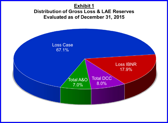
Exhibit 1 illustrates the types of reserves as a percent of our total reserve liability as of December 31, 2015. In 2015, 85.0% of our reserve liability (Loss case + Loss IBNR) was set aside to pay claimants, while 15.0% of our reserve liability (Total DCC + Total A&O) was established to accommodate costs associated with settling those claims. These costs are described in more detail later in this section.
We evaluate our total indicated loss reserve need by sorting and analyzing claims by accident date. This analysis, discussed in detail in Section VII of the Appendix, is completed concurrently with the evaluations of case and IBNR reserves for the same segmentation of business.
Loss case reserves represented 67.1% of our total carried reserves at December 31, 2015. Case reserves are estimates of amounts required to pay claims that have already been reported and recorded into Progressive’s systems, but have not yet been fully paid. We evaluate our indicated case reserve need, as discussed in Section VII of the Appendix, by sorting and analyzing claims by record date (the date the claim was recorded by the Company).
For each open claim, the Company carries a financial case reserve on its books. The financial case reserve is either an average reserve, determined by the Loss Reserving group or the adjuster reserve, which is our adjuster’s estimate of the remaining cost for the claim.
Average Reserves: Our objective is to use an average reserve for claims which we feel have a more predictable level of severity. We have determined a dollar threshold (which may vary by product, state, line coverage, and limit) under which a claim’s severity is sufficiently predictable to receive an average from Loss Reserving.
Page 7
Table of Contents
Adjuster Reserves: Our claims adjusters often will estimate the ultimate loss on a claim. We call this estimate the adjuster reserve. In cases where our adjuster sets a reserve equal to or above a pre-determined threshold, the adjuster reserve will be used to determine the financial case reserve rather than the average reserve.
When a claim is first recorded by the Company, there may not be enough known about the claim for an adjuster to determine its cost. The use of average reserves allows claims personnel to concentrate their efforts on adjusting claims rather than accounting for them. Also, average reserves are not as affected by changes in claims processes, and they provide more accurate financial reporting in aggregate.
Loss Reserving determines the average reserves, which vary by segment. In the months that a segment is not reviewed, an inflation factor is applied to the average reserves to keep up with changing costs between reviews. The inflation factor is generally based upon a projected future severity trend based on our analysis.
Once an average reserve is assigned to a claim, we monitor the age of a claim. The age of a claim is defined as the length of time from the accident date to the current accounting date. In certain coverages, such as Bodily Injury, more severe claims tend to remain open longer than less severe claims and tend to be more expensive due to litigation, medical treatments, and other associated costs. In order to recognize this cost differential, the average reserve increases as the claim ages for such coverages.
Our analysis has shown that all else being equal, claims recorded on time (i.e. immediately after occurrence) ultimately settle at a different average cost compared to claims recorded late. In order to recognize this cost differential, we began implementing a record-age segmentation to our case reserves in 2015.
Financial Reserves: The reserve carried on our books is the financial reserve. For claims in which the adjuster has not set a reserve, or for which the adjuster reserve has been set below the threshold, the average reserve from Loss Reserving is used as the financial reserve. If the adjuster reserve is set at or above threshold, however, the adjuster reserve is used as the financial reserve.
Severities may vary significantly on claims above the threshold. The adjuster reserves more accurately estimate the ultimate liability for these claims because the adjusters have typically spent a great deal of time on these larger claims and understand their unique characteristics. While only 14.8% of our total open claims count for Personal Auto Bodily Injury is set at or above the current threshold, these claims represent 33.6% of our total Personal Auto Bodily Injury case reserve liability as of year-end 2015. For Commercial Auto Bodily Injury, only 3.7% of our total open claim count is set at or above the threshold, accounting for about 31.1% of our total Commercial Auto Bodily Injury case reserve liability.
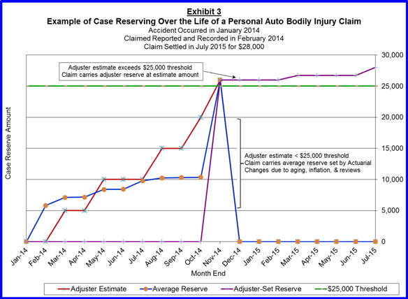
Example: Exhibits 2 and 3 illustrate the life of a hypothetical Personal Auto Bodily Injury claim. When the claim was originally recorded, we assigned the actuarially determined average reserve of $5,829. As the claim aged from the time it was reported in February through the end of October, the average reserve changed due to the application of the inflation factor, results of actuarial reserve reviews, and aging. Over this same period of time, the adjuster increased the reserve estimate (red line) multiple times as more information was obtained about the claim. When the adjuster’s estimate exceeded the sample threshold of $25,000, the financial reserve changed from an average reserve to an adjuster reserve.
Page 8
Table of Contents
Exhibit 2
Example of Loss Case Reserving Over the Life of a Personal Auto Bodily Injury Claim
Policy Limits = $30,000/$60,000
Threshold = $25,000
State XYZ
Inflation Factor = 6% per year
(Excludes Loss Adjustment Expenses)
| Month |
Claim Activity |
Age in Months* |
Adjuster Estimate |
Carried Reserve |
Amount Paid |
Explanation for Reserve Change | ||||||
| Jan-14 | Accident occurs | 1 | - | IBNR | - | Aggregate amount based on factor of EP for segment | ||||||
| Feb-14 | Claim is reported | 2 | - | 5,829 | - | Average reserve for 1-2 month age group from actuarial review | ||||||
| Mar-14 | Adjuster sets estimate | 3 | 5,000 | 7,121 | - | Aging to 3-4 month age group and inflation | ||||||
| Apr-14 | 4 | 5,000 | 7,157 | - | Inflation | |||||||
| May-14 | Adjuster revises estimate | 5 | 10,000 | 8,391 | - | Actuarial review and aging to 5-6 month age group | ||||||
| Jun-14 | 6 | 10,000 | 8,432 | - | Inflation | |||||||
| Jul-14 | 7 | 10,000 | 9,789 | - | Aging to 7-12 month age group and inflation | |||||||
| Aug-14 | Adjuster revises estimate | 8 | 15,000 | 10,250 | - | Actuarial review revised averages | ||||||
| Sep-14 | 9 | 15,000 | 10,300 | - | Inflation | |||||||
| Oct-14 | Adjuster revises estimate | 10 | 20,000 | 10,350 | - | Inflation | ||||||
| Nov-14 | Adjuster revises estimate | 11 | 26,000 | 26,000 | - | Adjuster estimate pierces threshold, so claim takes adjuster reserve | ||||||
| Dec-14 | 12 | 26,000 | 26,000 | - | ||||||||
| Jan-15 | 13 | 26,000 | 26,000 | - | ||||||||
| Feb-15 | 14 | 26,000 | 26,000 | - | ||||||||
| Mar-15 | Adjuster revises estimate | 15 | 26,725 | 26,725 | - | Still above threshold, so we continue to take adjuster reserve | ||||||
| Apr-15 | 16 | 26,725 | 26,725 | - | ||||||||
| May-15 | 17 | 26,725 | 26,725 | - | ||||||||
| Jun-15 | 18 | 26,725 | 26,725 | - | ||||||||
| Jul-15 | Claim is paid and closed | 19 | 28,000 | 0 | 28,000 | Carried reserve goes to zero as claim is closed with payment |
| Note: Age in Months = |
Number of Days since the Date of Loss |
rounded up to the nearest integer | ||
| 30 Days |
Page 9
Table of Contents
Incurred But Not Recorded (IBNR) Reserves
We establish a reserve for claims that have occurred, but have not been reported by the claimants or recorded by the Company as of the accounting date. IBNR Reserves are estimates of the amounts needed to pay these claims. At year-end 2015, the loss IBNR reserves were 17.9% of our total carried reserves.
The IBNR reserve need is evaluated by the same segmentation process used for case reserves. We perform this analysis by sorting historical claims according to the time lag between the accident dates and the dates that these claims were recorded by the Company. The case study in Section VII of the Appendix shows a detailed IBNR reserve analysis.
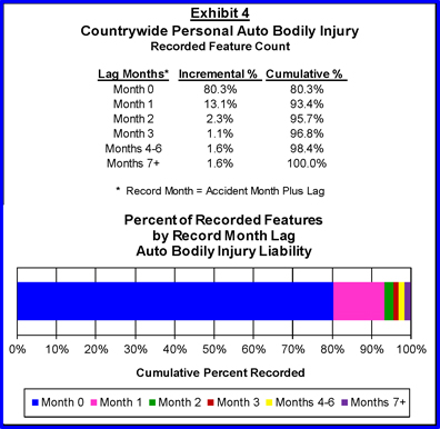
Late reported claims are evaluated to determine the estimated ultimate losses for each accident quarter within each lag period. For example, Lag month 1 consists of claims for which the accidents occurred during one month but were not recorded until the next calendar month. Similarly, Lag month 2 consists of all claims for which the accidents occurred during one month but were recorded by the Company two months later. Lag month 0 claims were recorded in the same month they occurred.
Exhibit 4 below shows our approximate percent of recorded features for Personal Auto Bodily Injury by record month lag. This exhibit shows 80.3% of our Auto BI features are reported and recorded in our systems by the end of the month in which they occurred. However, 19.7% of the features had not been recorded by the end of the accident month. Therefore, we need to estimate IBNR reserves for these claims.
Page 10
Table of Contents
The reserve analysis develops estimated IBNR factors based on the needed reserves by age divided by the earned premium for each age group. The carried IBNR reserves are calculated at the end of each month (by segment) by applying these IBNR factors to trailing periods of earned premium for up to four years. In almost all cases, the largest IBNR factors are applied to the premium in the most recent accident quarters because of their greater IBNR reserve need. The IBNR reserves change with our premium volume, allowing these reserves to keep up with growth, inflation, business mix, etc.
Loss Adjustment Expense (LAE) Reserves
In addition to loss payments (which indemnify claimants), the Company incurs expenses in the process of settling claims. Therefore, we need to establish a reserve liability to cover estimated LAE to be paid as loss reserves develop to closure. The two categories of LAE are DCC and A&O, which are defined4 as follows:
| Defense and Cost Containment (DCC) includes all defense, litigation and medical cost containment expenses, including in-house counsel. We evaluate the total indicated DCC expense reserve need by sorting and analyzing these expenses by accident date, similar to how we review the needed loss reserves. In addition to being analyzed in total, the DCC expenses are split into Attorney & Legal and Medical & Other components, which are analyzed separately. |
| Adjusting & all Other Expense (A&O) includes all other claims adjusting expenses, whether internal or external to the Company. A&O consists of fees, salaries and overhead expenses of those employees involved in a claim adjusting function, as well as other related expenses incurred in determination of coverage. We evaluate our total indicated A&O reserve need by taking A&O Charges to date and allocating them across states, products, coverages, and feature age. Based on this, we are able to create accident period triangles across the same segmentation. We generally create a triangle of total charged A&O and a triangle of the ratio of charged A&O dollars to Property Damage earned exposures. We then analyze and project these A&O costs to ultimate value, using development techniques that are discussed in more detail in the appendix. We then back out charged A&O to date from our ultimate projection to obtain our overall indicated A&O reserve. |
At year-end 2015, the LAE reserves were 15.0% of our total carried reserves. Similar to loss reserves, we carry case reserves for DCC and A&O expenses by applying selected averages to each open feature. For DCC, we carry the adjuster reserve if it exceeds a certain threshold, which occurs less frequently than for loss. Similar to loss IBNR reserves, carried DCC IBNR and A&O IBNR are calculated as a percentage of the trailing earned premium for each respective segment.
Analysis of needed DCC and A&O expense reserves are performed independently. For Personal Auto DCC Bodily Injury, we review reserves for each state at least once a year, though many states are not reviewed individually, but rather as part of a more aggregate review. We also review all A&O reserves by state and by line coverage at least once per year for Auto. For Commercial Auto the reviews are completed on a more aggregated basis. Section VIII of the Appendix contains a case study of our LAE reserve analysis.
4 The definitions are consistent with those prescribed by the NAIC under the Statutory Accounting Regulations
Page 11
Table of Contents
Involuntary Market Operating Loss Reserves
Progressive is required by the laws of most states to participate in involuntary market plans. Below we discuss the two major types of involuntary market plans in which we participate.
Private Passenger Assigned Risk Plans: Certain state insurance regulations require us to participate in various assigned risk plans. Applicants who cannot obtain insurance in the voluntary market are assigned to insurers in proportion to the volume of written exposures or vehicles each insurer writes in that state. Historical data indicates an operating loss is to be expected on these assignments. Participation requirements in assigned risk plans differ from state to state. Reserves are established for these expected operating losses based on our current written exposures. Since the plans assign business to policy years two years in the future based on our current writings, we carry the reserves until we are actually assigned the risks.
The carried reserves for assigned risk plans comprised less than one-tenth of one percent of our total net carried reserves at year-end 2015. However, since this is a unique type of exposure, we evaluate it separately.
The process of determining the assigned risk reserve for a state is as follows:
| ● | Determine Progressive’s estimated portion of the assigned risk pool by multiplying our projected market share by the estimated future size of the assigned risk pool in that state |
| ● | Reduce this by any credits a state may allow such as voluntarily writing risks that generally populate the plans in a higher portion than in the general market |
| ● | Estimate the operating loss that we expect to incur from this business |
| ● | Factor in the impact when excess credits are sold to competitors along with charges from Limited Assigned Distribution (LAD) carriers when such agreements are in force |
Commercial Auto Insurance Procedure (CAIP): In most states, Progressive is also required to share in the operating results of the involuntary CAIP plan. Due to the more complex nature of commercial business, these plans do not assign policies to specific insurance companies. Instead, a small number of carriers (including Progressive) service the business, but generally do not bear underwriting risk. The servicing carriers transfer the insurance risk, or cede 100% of the business, to the state pools. These pools then retrocede the loss experience of the plan to all companies in proportion to their respective shares of the commercial automobile voluntary market for the respective state.
Other Considerations to Reserves
Salvage and Subrogation
GAAP requires loss reserves to be stated net of anticipated salvage and subrogation recoveries. Statutory Accounting Principles (SAP), which are mandated by state insurance departments or regulators, allows reserves to be reduced by the expected recovery amounts but does not require it. We report our SAP loss reserves net of anticipated salvage and subrogation recoveries.
Salvage: Progressive generally assumes the title to a vehicle when it is declared a total loss. We may then sell the vehicle to a salvage dealer and these proceeds net of expenses are referred to as salvage recovery. Salvage is most relevant in analyzing the needed reserves for Collision claims.
Subrogation: When a Progressive policyholder is involved in an accident in which the other party is at fault or partially at fault, he or she may submit the claim to us. When we pay that claim, we obtain our policyholder’s right to recover damages from the at-fault party or the at-fault party’s insurance company. Subrogation is most relevant for Collision claims (damage to our insureds’ vehicles) and Personal Injury Protection (PIP) claims.
Page 12
Table of Contents
As we collect salvage or subrogation from third parties, it reduces our net paid and incurred loss amount for that claim. We analyze our claims data net of these recoveries, so that our estimated ultimate loss amounts are net of anticipated salvage and subrogation. Since most of our recoveries are realized after claims have been closed, we may carry negative IBNR reserves on the Company’s books for anticipated future recoverable salvage and subrogation.
Catastrophes
The United States does not allow insurance companies to set up reserves for catastrophes ahead of time due to accounting and tax principles. An event/storm is declared a catastrophe by an external agency if the industry wide total insured losses will amount to more than $25 million. The type of loss will vary depending on the type of storm. For example, losses from a hurricane will be different than losses from a hail storm or a forest fire.
Progressive predicts its total comprehensive losses for a catastrophe by looking at data from prior storms. Specifically, we will look at prior storms’ development factors, frequency and severity. If a catastrophe occurs too close to the end of the month, there is less time for claims to be reported, and therefore we may put up IBNR reserves to cover the additional amount we think we will need for the total amount of losses. We also know that we will receive some amount of salvage, and we factor this into the projection for total losses.
Page 13
Table of Contents
Section III – About Reserves and Development
In order to measure how well we are achieving our stated goals, we track the development of reserves from the time they are initially booked until losses are fully developed. In order to understand how reserve development impacts Progressive’s financial statements it is important to understand the difference between Calendar Period and Accident Period data.
Calendar Period versus Accident Period
Financial statements report data on a calendar period basis. However, payments and reserve changes may be made on accidents that occurred in prior periods, thus not giving an accurate picture of the business that is currently insured. Therefore, it is important to understand the difference between calendar period and accident period losses.
Calendar Period Losses consist of payments and reserve changes that are recorded on the Company’s financial records during the period in question, without regard to the period in which the accident occurred. Calendar period results do not change after the end of the period, even as new claim information develops.
Accident Period Losses consist of payments and reserves for losses that occurred in a particular period (i.e., the accident period). Accident period results will change over time as the estimates of losses change due to payments and reserve changes for all accidents that occurred during that period.
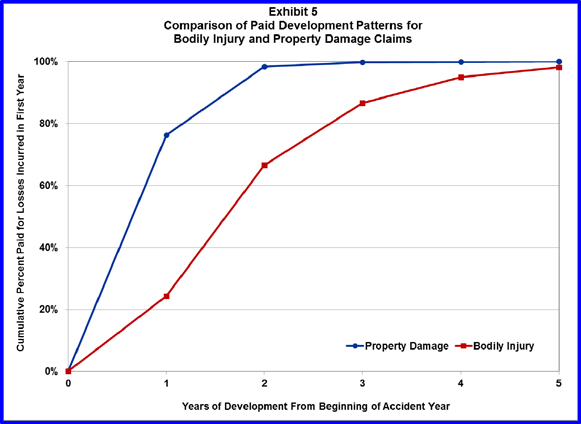
Incurred losses consist of payments and reserve changes, so it is important to understand paid development patterns. The longer a claim is expected to stay open (not settled), the more difficult it is to establish an accurate reserve at the time the accident is reported. Since injury claims tend to take longer to settle than property claims, total reserve estimates for injury claims are more sensitive to the uncertainties mentioned above, such as changes in mix of business, inflation, and legal, regulatory or judicial issues. As more information is obtained about open claims, the reserves are revised accordingly. The ultimate amounts, however, are not known until the claims are settled and paid.
The following chart (Exhibit 5) compares the time it takes to settle a typical segment of Bodily Injury liability claims versus a typical segment of Property Damage liability claims. Each annual development point represents the cumulative percent of paid dollars for accidents that occur in the first year.
Page 14
Table of Contents
The ultimate paid losses (i.e., our projection of fully-developed paid losses) and ultimate LAE may deviate, perhaps substantially, from point-in-time estimates of reserves contained in our financial statements. The actual claims payments in subsequent calendar years may exceed or may be less than the year-end carried loss reserves causing losses incurred in subsequent calendar years to be higher or lower than anticipated. Changes in the estimated ultimate cost of claims are referred to as development.
There are several ways for reserve development to occur:
| ● | Claims settle for more or less than the established reserves for those claims. |
| ● | Adjuster reserve estimates on open (reported) claims change, such that a claim previously set below threshold is now set at or above the threshold (or vice versa). |
| ● | Average reserves set by Loss Reserving for open (reported) claims change |
| ● | Unrecorded claims emerge (i.e., they are recorded after the accounting date) at a rate greater or less than anticipated. This can be due to either or both of the following: |
| ¡ | The actual number (frequency) of “late reported” claims differs from the estimate |
| ¡ | The average amount (severity) of these claims differs from the estimate |
| ● | Loss Reserving’s estimates of future emergence patterns on unreported claims change |
| ● | Salvage and subrogation recoveries are greater or less than anticipated |
| ● | Changes in earned premium affect carried IBNR (incurred but not recorded) reserves which are calculated as a percentage of earned premium |
Page 15
Table of Contents
Exhibit 6 illustrates Progressive’s reserve development over the past ten years. It shows the booked reserves at each year-end, and the re-estimated needed reserves at each subsequent year-end (down the column for each original accounting date). The last diagonal (in red) in Exhibit 6 represents our evaluation, as of December 31, 2015, of the needed reserves as of each respective year-end. The difference between the current evaluation (last diagonal) and the original amount of booked reserves in each column represents cumulative reserve development for that accident year and all prior accident years combined. This measures our performance against the goal, stated above, that total reserves are intended to be adequate and to develop with minimal variation.
|
Exhibit 6 Analysis of Loss and Loss Adjustment Expense (LAE) Development (in millions) (unaudited) | ||||||||||||||||||||||||||||||||||||||||||
|
For years ending Dec. 31, |
2005 | 2006 | 2007 | 2008 | 2009 | 2010 | 2011 | 2012 | 2013 | 2014 | 2015 | |||||||||||||||||||||||||||||||
|
Net Loss & LAE reserves |
$5,313.1 | $5,363.6 | $5,655.2 | $5,932.9 | $6,123.6 | $6,366.9 | $6,460.1 | $6,976.3 | $7,433.8 | $7,893.9 | $8,596.3 | |||||||||||||||||||||||||||||||
| Re-estimated reserves, as of |
|
|||||||||||||||||||||||||||||||||||||||||
| One year later |
$5,066.2 | $5,443.9 | $5,688.4 | $5,796.9 | $5,803.2 | $6,124.9 | $6,482.1 | $7,021.4 | $7,409.7 | $7,578.8 | ||||||||||||||||||||||||||||||||
| Two years later |
$5,130.5 | $5,469.8 | $5,593.8 | $5,702.1 | $5,647.7 | $6,074.4 | $6,519.6 | $6,994.7 | $7,402.4 | |||||||||||||||||||||||||||||||||
| Three years later |
$5,093.6 | $5,381.9 | $5,508.0 | $5,573.8 | $5,575.0 | $6,075.9 | $6,495.4 | $6,983.2 | ||||||||||||||||||||||||||||||||||
| Four years later |
$5,046.7 | $5,336.5 | $5,442.1 | $5,538.5 | $5,564.6 | $6,050.6 | $6,459.8 | |||||||||||||||||||||||||||||||||||
| Five years later |
$5,054.6 | $5,342.8 | $5,452.8 | $5,580.0 | $5,605.6 | $6,097.4 | ||||||||||||||||||||||||||||||||||||
| Six years later |
$5,060.8 | $5,352.8 | $5,475.6 | $5,609.1 | $5,638.8 | |||||||||||||||||||||||||||||||||||||
| Seven years later |
$5,070.2 | $5,369.7 | $5,501.3 | $5,634.9 | ||||||||||||||||||||||||||||||||||||||
| Eight years later |
$5,081.7 | $5,391.2 | $5,527.1 | |||||||||||||||||||||||||||||||||||||||
| Nine years later |
$5,100.6 | $5,406.4 | ||||||||||||||||||||||||||||||||||||||||
| Ten years later |
$5,110.2 | |||||||||||||||||||||||||||||||||||||||||
| Cumulative Development: |
||||||||||||||||||||||||||||||||||||||||||
|
favorable/(unfavorable) |
$202.9 | ($42.8) | $128.1 | $298.0 | $484.8 | $269.5 | $0.3 | ($6.9) | $31.4 | $315.1 | ||||||||||||||||||||||||||||||||
|
% of Original Reserves |
3.8% | -0.8% | 2.3% | 5.0% | 7.9% | 4.2% | 0.0% | -0.1% | 0.4% | 4.0% | ||||||||||||||||||||||||||||||||
The reserves set as of December 31, 2014 appeared to be adequate as of year-end 2015, since reserves developed favorably over the course of 2015. In other words, as of year-end 2015, we estimate that claims will cost less than what we projected at year-end 2014. Recall that excessively adequate or deficient reserves can, respectively, limit competitive opportunities or cause unprofitable growth. It is important to recognize both favorable and unfavorable development as quickly as possible, so that these inefficiencies are corrected and our financial results are presented as accurately as possible.
As seen in Exhibit 6, we have developed favorably year-to-date for most year-end evaluations except 2006 and 2012. We experienced cumulative development of 5% or more for 2008 and, 2009. In contrast, the cumulative reserve development for 2005, 2007, 2010, 2011, 2013, and 2014 was favorable, but much more modest in magnitude. For these years, reserves have run-off between 0.005% and 4.2% of the originally-held amount. Reserves for 2006 and 2012 experienced modest unfavorable development. Exhibit 6 quantifies the amount of favorable development in 2015 at the bottom of the 2014 column. Reserves from accident years 2014 and prior developed favorably by $315.1 million, representing 4.0% of the originally held reserves or 1.6% of our 2015 earned premium ($19.9 billion, found on page 18).
We make many projections in loss reserve analyses that may change as the claims mature. The least mature claims are those that occurred during the most recent accident year, so the Company believes that the estimated severity for the 2015 accident year is the projection with the highest likelihood to change. For further discussion of the 2015 results and how they are affected by loss and LAE reserves, see “Management’s Discussion and Analysis of Financial Condition and Results of Operations” in the Company’s 2015 Annual Report to Shareholders, which is attached as an appendix to the Company’s 2016 Proxy Statement.
Page 16
Table of Contents
Reserve development influences our reported earnings. Reported earnings for any period may be understated (relative to accidents that occur in that period) when either or both of the following items occur:
| ● | There is unfavorable development of prior accident years during the current period |
| ● | Reserves for accidents that occur in the current period are overestimated (i.e., subsequent evaluation shows a lower estimate of ultimate incurred losses) |
On the other hand, reported earnings for any period may be overstated when the opposite of these items occurs.
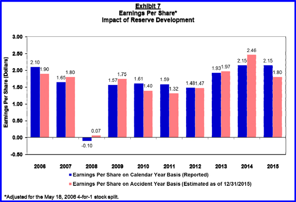
Exhibit 7 shows how reported Earnings Per Share (EPS) are affected by the reserve development in Exhibit 6. It shows the reported EPS for specified fiscal years and what the EPS would have been if the Company had had no reserve development, i.e., if the specific year’s earnings were based on only that year’s accidents. Each specific year’s adjusted EPS excludes prior accident years’ development during the specific year and includes future development of the current accident year, estimated as of year-end 2015. For example, it can be seen in Exhibits 6 and 7 that in calendar year 2015 reserves developed favorably. Note that the negative EPS in 2008 was driven by losses in the investment portfolio.
External Reporting of Reserve Changes and Reserve Development
Since reserve changes affect calendar period earnings, our monthly earnings release shows actuarial reserve changes by Personal Lines (Agency and Direct), Commercial Lines, and Property. We also report reserve development monthly, in addition to the quarterly and annual reporting requirements. This information for the current month and year-to-date is included in the “Supplemental Information” section of our monthly earnings release. The following excerpt is from our December 2015 earnings release and is unaudited:
Page 17
Table of Contents
| December 2015 Year-to-Date ($ in millions) |
Companywide Total | |
| Net Premiums Earned |
$19,899.1 | |
| Actuarial Adjustments |
||
| Reserve Decrease/(Increase) |
||
| Prior accident years |
$95.1 | |
| Current accident year |
97.0 | |
| Calendar year actuarial adjustment |
$192.1 | |
| Prior Accident Years Development |
||
| Favorable/(Unfavorable) |
||
| Actuarial adjustment |
$95.1 | |
| All other development |
220.0 | |
| Total development |
$315.1 | |
| Calendar year loss/LAE Ratio |
72.1 | |
| Accident year loss/LAE Ratio |
73.7 | |
The table shows that we decreased our loss and LAE reserves during 2015 by $192.1 million as a result of regularly scheduled actuarial reviews. Each month, we generally complete between 50 and 75 reviews, representing slightly more than 25% of our total amount of reserves. Some reviews result in needed changes to the carried reserves. The total change is reported as Actuarial Adjustments in the table. A reserve decrease is shown as a positive value on the earnings report because it increases our earnings for the reporting period.
Actuarial adjustments decreased reserves for accident year 2015 by $97.0 million, while reserves for claims in prior accident years were decreased by $95.1 million. However, this actuarial reserve decrease, which applies to claims in prior accident years, represents only one portion of the prior year development.
As stated earlier in this section, favorable or unfavorable development is due to a combination of factors. The favorable actuarial adjustment of $95.1 million includes changes to averages on open claims and the estimated emergence of claims that were unreported as of prior year-end. The all other favorable development of $220.0 million includes claims settling for amounts different from the established reserves, changes to adjuster reserves, actual emergence of claims that was different than the expected emergence included in IBNR reserves, and salvage and subrogation recoveries greater or less than expected.
The total prior accident years’ development listed above ties back to the cumulative development listed in Exhibit 6. Through December 31, 2015, including actuarial adjustments and all other development, the total prior accident years’ development was favorable by $315.1 million. In other words, with updated information as of December 31, 2015, we estimated that our reserves as of December 31, 2014 should have been $315.1 million lower than they were.
The $315.1 million favorable prior accident years’ development during 2015 is included in our calendar results for 2015. As a result, our 2015 calendar year incurred loss and LAE ratio of 72.1% is lower than our 2015 accident year incurred loss and LAE ratio of 73.7%. The difference of 1.6 points reflects the $315.1 million favorable development through December 31, 2015 divided by the net earned premium of $19.9 billion for the same period.
Reserve changes made as a result of actuarial reviews are intended to keep our current reserve liability accurate for the business reviewed. We change the reserves for the reviewed business
Page 18
Table of Contents
based upon current information and our projections of expected future development. This is not the same as the aggregate development of prior year-end reserves.
Internal Reporting of Reserve Changes and Reserve Development
After completing each segment review, Loss Reserving analysts send summaries of the reviews to all affected areas of the Company. Loss Reserving meets with Product Management, Pricing, and Claims to discuss the current change, development, trend, and other issues that were considered in reserve analysis and exchange information that may be considered in future reviews. The participation of these business units allows Loss Reserving to better understand changes in processes and business operations that may be affecting the underlying data.
To help Product Management understand the case reserve changes shown on their income statements, we provide a monthly Decomposition Report that summarizes the changes in the following categories (terms are explained in Sections II and VI):
| ● | features that closed |
| ● | features that opened (including reopened features) |
| ● | changes in reserve averages on new features (due to loss reserving) |
| ● | changes in reserve averages on open features (due to loss reserving) |
| ● | inflationary impact on open features (inflation factor applied to average reserves) |
| ● | aging of open features (features moving to the next age group) |
| ● | changes from adjuster reserve to average reserve (reserve amount changes from above threshold to below threshold) |
| ● | changes from average reserve to adjuster reserve (reserve amount changes from below threshold to above threshold) |
| ● | changes in adjuster reserves (reserve amount changes, but stays above threshold) |
| ● | changes due to re-segmentation of data |
The business units are also provided with updated information regarding the impact of prior accident years’ development on their current calendar year results. We track the reserve development on prior accident years, which allow us to retrospectively test our prior assumptions and apply that knowledge in future judgments. It also helps the Product Managers to better understand how their calendar year earnings are affected by reserve development.
Page 19
Table of Contents
Section IV – Estimating Loss Reserves
During a reserve review we generally estimate the ultimate loss amounts for the past seven accident years using up to six different projections (discussed in more detail below). We may use additional techniques if there are wide variations between the various projections or if underlying process changes make those projections less reliable. To estimate the required reserve balance (i.e., unpaid losses) for the segment, we subtract the payments we have already made on claims that occurred during that same period. We change the reserve level for that segment based upon this review.
In this section, we discuss segmentation and describe the projections we consider in the review. The Appendix contains case studies that show more details involved in the segment reviews, including the calculations and the issues involved in performing the reviews. However, the application of judgment is a key component of our reserve analysis and decisions on the necessary reserve changes. This is especially true in dynamic environments such as those we have experienced at Progressive, in which changes in mix of business (e.g., by policy limit and geographic area) can be significant.
Segmentation of Reserves for Analysis
Segments are identified to allow us to review reserve needs at the most detailed level our data supports, and provide us with the ability to identify and measure variances and trends in severity and frequency. They also allow us to identify process changes within states/regions, which helps us to understand changes within the underlying data and to reflect them in the reviews. Each segment is generally required to have enough data to deliver reliable (credible) results. Our objective is to achieve adequacy in the reserve levels with minimal variation for each segment. This enhances the accuracy of our financial reporting, supports the income statements of our business units, and allows us to make better business decisions.
The projection of frequency for the lines of business we write is usually stable even though actual frequency experienced will tend to vary depending on external factors. Examples include change in the mix of classes of drivers we insure, weather, or economic pressures like the price of gas. The severity experienced by the Company is more difficult to estimate, and it is affected by changes in underlying costs, such as medical costs, jury verdicts, etc. In addition, severity will vary based on the change in the Company’s mix of business by policy limit or deductible.
Internal and external considerations are better understood at the state level than at a more macro countrywide level. Internal considerations that are process-related may result from changes in the claims organization’s activities, including claim closure rates, the number of claims that are closed without payment, and the level of estimated needed case reserves by claim. External considerations include the litigation environment, regulatory and legislative actions, state-by-state changes in medical costs, and the availability of services to resolve claims.
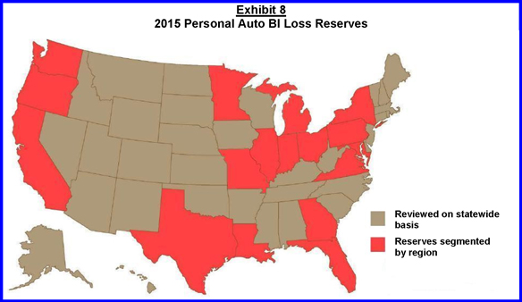
Due to our volume, we review each state separately for Personal Auto Bodily Injury loss reserves. Even though a few of these states may be considered too small to have fully credible data, we feel there is value in studying and interpreting each individual state’s trends and development. Some states are so large that we can segment the data into regions within the state. Exhibit 8 is a map showing how we currently segment our loss reserve reviews for Personal Auto Bodily Injury.
For some coverages, where the underlying data is not large enough to be credible, we may combine states with similar loss characteristics and review them together. We continually look at ways to further segment our reviews to add value to our process. Examples include enhanced accuracy and information provided to our Product Management and Pricing groups.
Page 20
Table of Contents
With respect to Personal Auto Bodily Injury and Uninsured Motorist coverage, we split loss data into groups based on policy limits and analyze the data. It is valuable to analyze these groups of segments, as they tend to have different severity, frequency and loss development patterns. We also split the data by policy limit for our Commercial Auto Bodily Injury analyses (Specialty truck is analyzed separately from Business Auto). Each identified segment is reviewed annually, semiannually, or quarterly depending on the size, the volatility, and other unique aspects of the individual segment. As the need to further analyze expenses at a finer breakout by limit presents itself, we have structured these more in-depth reviews.
LAE reserves are analyzed at a level of segmentation using many of the same considerations as loss reserves. Since the volume of LAE reserves is much less than that of loss reserves, we combine most of the states for Auto DCC reviews for coverages other than Bodily Injury and PIP. This produces more credible results. A&O is reviewed by state for all Auto line coverages. As mentioned earlier, all LAE segments are evaluated at least once per year, generally twice. Commercial Auto is also broken out similar to Auto for LAE, but not to the same level of geographic detail.
Projections of Ultimate Losses
Our standard procedures are to review the results of the different projections in order to determine if a reserve change is required. Three of the six available projections use paid data and the other three projections use incurred data (payments plus case reserves). There are strengths and weaknesses to each of the projections. In the event of a wide variation between results generated by the different projections, we further analyze the data using additional techniques.
The six available standard projections we use to estimate ultimate losses are:
| 1. | Amount Paid, in which we organize the total loss dollars paid by accident period and age of development into a triangular format (refer to Exhibit B of the Appendix) and project them to estimated ultimate amounts. We base our selections of future expected loss development largely on the historical development of prior periods. |
Page 21
Table of Contents
| 2. | Average Paid, in which we organize the paid severity (average amount paid per feature) by accident period and age of development into a triangular format and project the severities to estimated ultimate levels. Ultimate loss amounts are then calculated as the ultimate severities multiplied by the estimated ultimate number of features to be paid. |
| 3. | Bornhuetter-Ferguson Paid, which uses the paid loss development pattern to determine the percent unpaid. We apply the percent unpaid to the expected ultimate loss amount to arrive at the expected unpaid amount, which is added to actual losses paid-to-date. |
| 4. | Amount Incurred, in which we organize the total loss dollars incurred by accident period and age of development into a triangular format and project them to estimated ultimate amounts. We base our future expected loss development largely on the historical development of prior periods. |
| 5. | Average Incurred, in which we organize the incurred severity (average amount incurred per feature) by accident period and age of development into a triangular format and project the severities to estimated ultimate levels. Ultimate loss amounts are then calculated as the ultimate severities multiplied by the estimated ultimate number of features to be paid. |
| 6. | Bornhuetter-Ferguson Incurred, which uses the incurred loss development pattern to determine the percent not yet recorded. We apply the percent unrecorded to the expected ultimate losses to arrive at the expected unrecorded amount, which is added to actual losses incurred-to-date. |
The three paid projections – amount paid, average paid, and Bornhuetter-Ferguson paid – all use paid loss data. The paid projections estimate growth and development of claims in an accident period by looking at the paid development of earlier accident periods. This assumes that past paid loss development is a predictor of future paid loss development. The primary strength of using paid data is that it removes the potential for distortions that may be created by including estimated data (i.e., case reserves). The drawback is that it is more difficult to accurately project ultimate losses in the most recent periods under review. For example, with longer-tailed lines of insurance such as Bodily Injury, the early development periods are more volatile because a large proportion of the payments are made later, as was illustrated in Exhibit 5 of Section III. Accurate paid projections also depend heavily on consistent claims closure or settlement practices. If the closure rate changes, the paid projections could be misleading. In addition, shifts in mix of business (e.g., changes by policy limit) are not as readily identified in the past paid development as in the incurred loss development.
The three incurred projections – amount incurred, average incurred, and Bornhuetter-Ferguson incurred – use paid losses plus case loss reserves in each accident period. They assume that historical incurred loss development will be predictive of our future incurred loss development. The primary strength of using incurred data is that we can make use of reserve estimates for open claims. These estimates are based on the judgment of claims adjusters, in addition to our prior actuarial reviews. This is especially critical when estimating ultimate losses for longer-tailed claims such as Bodily Injury. The drawback of using incurred data for projection is that it depends heavily on adjusters using consistent reserving practices, which can vary over time.
We study changes in closure rates and average adjuster reserve levels through our segmentation of data and also through discussions with management. We adjust for these changes in our projections of losses. The case study in Section VII of the Appendix includes more thorough explanations of how changes in the closure rate affect paid loss development, and how changes in average adjuster reserves affect incurred loss development.
For the year, we conducted 729 reviews involving 328 segments of business.
Page 22
Table of Contents
ARX Holding Corporation
On April 1, 2015, Progressive acquired a controlling interest in ARX, the parent company of one of our Progressive Home Advantage (PHA) partners, American Strategic Insurance (ASI). As of this writing, Progressive owns about 69% of ARX Holding Corporation, with an agreement in place providing the right to acquire 100% ownership within six (6) years from the date of acquisition.
ARX’s business is primarily made up of Homeowners insurance, which is a short-tailed coverage. Homeowners and dwelling/fire accounts for approximately 90% of the carried reserves. The remaining 10% is made up of umbrella and commercial multi-peril. Both the personal lines and commercial lines are heavily reinsured, with the intent of providing ARX with increased capacity to write larger risks while maintaining exposure to losses within its capital resources.
ARX reviews data on a monthly basis, segmented by product, annual statement line, and state. Standard actuarial techniques, including Paid, Incurred, Average Paid, Average Incurred, Bornhuetter-Ferguson Paid, and Bornhuetter-Ferguson Incurred, which are described on pages 21-22, are reviewed.
Page 23
Table of Contents
Accident Period Losses: Losses for each accident are assigned to the period in which the accident occurred. Accident periods used in our analysis are generally three months (accident quarter), six months (accident semester), or twelve months (accident year). Payments and reserve changes, regardless of when they are made, are assigned to that same period in which the accident occurred. Therefore, accident period results will change over time as the losses develop.
Adjuster Reserves: See Case Reserves.
Adjusting & All Other Expense (A&O): A component of loss adjustment expense. A&O expenses include all claims adjusting expenses (whether internal or external to the Company) that are not included in Defense and Cost Containment (DCC). This category includes fees and salaries of those involved in a claim’s adjusting function, and other related expenses incurred in determination of coverage. Adjusting and Other expense reserves are a bulk reserve, meaning they are not attributable to any specific feature or claim. A&O is sometimes called “AOE” outside of Progressive.
Assigned Risk: People unable to obtain auto insurance in the voluntary market apply for coverage in the state automobile plan. In most cases, the insurance coverage is not actually provided by the state but instead is “assigned” to an insurance company. Each insurance company is required in most states to accept a share of these risks proportionate to its volume of business in any given state.
Average Reserves: See Case reserves.
Bodily Injury (BI) Liability Coverage: Covers legal liability arising from an insured who causes injury or death to another person while using the insured vehicle. In most states, this is a mandatory coverage. Each state mandates the minimum required limit. BI coverage pays when our insured is liable for an accident in which another party is injured.
Bornhuetter-Ferguson Method: The “BF” method is an actuarial methodology that calculates the projected ultimate losses using a blend of a pure incurred or paid development method and an expected loss ratio (or expected pure premium) method.
Business Auto Commercial Vehicles: Commercial vehicles that generally have a gross vehicle weight under 26,000 pounds. These vehicles are used in the insured’s business but are not the primary source of revenue for the business.
Calendar Period Losses: Payments and reserve changes which are recorded in the Company’s financial system during the period in question, without regard to the period in which the accident occurred or was recorded. Calendar period results do not change after the end of the period, even as new claim information develops.
Case Reserves: Estimates of amounts required to settle claims that have already been recorded but have not yet been closed. Case reserves represent the largest portion of the reserves for automobile insurance products. The case reserves carried on the Company’s financial records are called the financial case reserves.
| ● | Adjuster Reserves: The claims adjuster’s best estimate of how much a specific claim will cost (or the average reserve, if the claims adjuster does not make an estimate). If the estimate is above a predetermined threshold, it is used to determine the financial case reserves. All adjuster reserves are included in the actuarial reserve analyses. |
Page 24
Table of Contents
| ● | Average Reserves: When the adjuster estimate for a feature is below a predetermined threshold, the financial case reserve is the average reserve. These are determined by the Loss Reserving group and vary by segment. Within each segment, they may also vary by age (months since the accident occurred), policy limit, and geographic area. |
| ● | Financial Case Reserve: The reserve carried on the books for an open claim. This amount is equal to the average reserve if there is no adjuster reserve, or if the adjuster reserve is below the threshold. If the adjuster sets a reserve at or above threshold, then that amount is taken as the financial reserve. |
Catastrophe: A term applied to an incident, storm or series of related incidents resulting in a significant number of claims with a combined cost totaling more than $25 million in property damage for the insurance industry.
Cede: To transfer liability, or a portion of it, in connection with a risk from the original or primary insurer to a reinsurance entity (e.g. a reinsurance company or Joint Underwriting Association).
Claim: A demand for payment by an insured or an alleged third party under the terms and conditions of an insurance contract.
Claimant: Usually refers to one who makes a claim.
Closed Without Payment (CWP): A claim that was reported, did not require a loss payment, and is now closed. Note that there can be loss adjustment expenses for a CWP claim.
Closure Rate: The number of claims from a specific accident period which are closed with payment at a specific evaluation date, divided by the estimated ultimate number of claims to be paid for that accident period.
Collision Coverage: A coverage of the automobile insurance policy that indemnifies the insured when his/her automobile is damaged due to physical contact with another object (except a bird or animal), or due to upset (e.g., overturning).
Combined Ratio: The sum of the loss and loss adjustment expense ratio and the expense ratio. This represents the percentage of each premium dollar an insurer spends on claims and expenses. A combined ratio less than 100% indicates an underwriting profit, while a combined ratio in excess of 100% indicates an underwriting loss.
Comprehensive Coverage: A coverage of the automobile insurance policy that pays for damages to the insured’s vehicle due to any cause (except collision), including damage due to fire, windstorm, hail, theft, falling objects, explosion, riot, glass breakage and other causes of loss.
Credibility: A statistical measure of the ability to infer generalizations from a data sample. Credibility increases as sample size increases or variability within the sample decreases.
Decomposition (Decomp) Reports: Monthly internal management reports that decompose the financial case reserve changes into categories that explain the reasons for the changes.
Defense and Cost Containment (DCC) Expense: A component of loss adjustment expense. DCC includes expenses related to defense, litigation and medical cost containment whether internal or external to the Company. DCC expenses include but are not limited to accident investigation, surveillance, litigation management, and fees of attorneys and others if working in defense of a claim.
Development: Change in the estimated or actual losses or reserves over subsequent evaluations. When compared to expectations or prior estimates, it is referred to as either
Page 25
Table of Contents
favorable or unfavorable development, based on whether the estimate has decreased or increased.
Development factor: The quotient of the paid or incurred value for an accident or record period evaluated at time t divided by the value for that same accident or record period evaluated at time (t – 1).
Diagonal: The cumulative or incremental values or factors for all accident or record periods being evaluated as of a common date. If we are evaluating accident semester paid losses at 6-month intervals, then the last diagonal of the paid loss triangle is made up of the cumulative paid loss amounts for each accident semester as of the most recent evaluation date. The development of that last diagonal would be the paid losses during the last six calendar months for each accident semester. (Also see Triangle).
Earned Car Year: An exposure unit that is the basic rating unit underlying an auto insurance premium. One automobile insured for a period of twelve months is one earned car year.
Earned Premium: That part of the premium proportional to the segment of time a policy has been in force. It is the premium for protection actually provided during the experience period.
Economic Capital: The amount of capital that a business needs to ensure that it remains solvent. It is a measure of risk, not of actual capital available to the business.
Emergence: Generally used in the context of IBNR reserves, it refers to the recording of claims (or dollar amount of the claims) after the date of the accident, usually into at least the next quarterly or annual period. For example, if an accident occurred in October 2012 and it was recorded in February 2014, it was part of the estimate of IBNR at year-end 2012, and it emerged in the first quarter of 2014.
Expense Ratio: The sum of all underwriting and operational expenses divided by premium. These expenses include such items as commission, acquisition expenses, general expenses, and taxes, but not LAE.
Exposure: A measure of the risk of loss and the basic rating unit underlying an insurance premium. The unit of exposure will vary based upon the characteristics of the insurance coverage involved. For automobile insurance, one automobile insured for a period of twelve months is one earned car year or one exposure.
Feature: The smallest divisible part of a claim. This is a loss on one coverage for one person or one property. Often a claim will involve multiple features. It can involve multiple coverages, such as Bodily Injury (BI), property damage (PD), and Collision; and/or it can involve multiple claimants for the same coverage (e.g., two injured parties).
Financial Case Reserves: See Case Reserves.
Frequency: Number of features divided by exposure count. If one exposure is defined as one earned car year, then frequency is a measure of the proportion of insureds that have a claim in a year.
Incurred But Not Recorded (IBNR) reserves: These are estimates at a given evaluation date of amounts that will be needed to settle claims that have already occurred but have not yet been recorded by the Company.
Incurred Losses: The sum of payments and case reserves.
Indication: An actuarial estimate, based upon analysis of the data.
Page 26
Table of Contents
Lag: Generally used in the context of IBNR reserves, it refers to the period of time from the date of the accident to the date the claim is recorded on the Company’s books. The data is grouped into quarterly and annual lag periods for analysis of IBNR reserves.
Loss Adjustment Expenses (LAE): Expenses related to claim settlement.
Total Loss Adjustment Expenses (LAE) =
[Defense and Cost Containment (DCC) expenses] + [Adjusting & Other (A&O) expenses]
Loss Adjustment Expenses (LAE) ratio: LAE expenses divided by earned premium.
Loss ratio (Incurred loss ratio): Incurred losses divided by earned premium.
Loss Reserving Segment: See Segment.
Net Loss Reserves: Net indicates that we have deducted the expected reinsurance recoverable from the sum of case and IBNR reserves. It may also refer to reserves that have been reduced for expected salvage and subrogation recoveries.
No-Fault Insurance: A type of insurance contract under which an insured is indemnified for losses by their own insurer, regardless of fault in the accident generating the loss, and limited in the right to seek recovery through the civil-justice system for losses caused by other parties.
Paid Losses: Payments for claims.
Parameters: Variables that determine the characteristics or behavior of a statistical model and can be estimated by calculations from sample data. For example, the parameters of frequency and severity are estimated in the loss reserve analysis model.
Personal Injury Protection (PIP) Coverage: Coverage in which an insurer pays, within specified limits, the medical and funeral expenses, work loss benefits and essential services of the insured, others in his vehicles and pedestrians struck by him. The basic coverage is implemented under no-fault automobile statutes, which vary by state.
Physical Damage: Damage to the insured vehicle, which includes the comprehensive and collision coverages.
Property Damage (PD) Coverage: A coverage that pays the legal liability of the policyholder for damage to, or destruction of, property of others in an auto accident, including damage to other vehicles and structures such as buildings, telephone poles and fences.
Pure Premium: Loss dollars divided by exposure count. Pure premium is also equal to frequency times severity. The pure premium is equivalent to the loss component of the full policy premium.
Record Period Losses: Losses are assigned to the period in which the accident is recorded on the Company’s financial records. Record periods used in our analysis are generally three months (record quarter), six months (record semester), or twelve months (record year). Payments and reserve changes, regardless of when they are made, are assigned to that same period in which the accident was recorded. As a result, record period results will change over time as the losses develop, i.e., as the estimates of losses change due to payments and reserve changes for all accidents that were recorded during that period.
Reopened Claim: A claim that was closed (with or without payment) but opened again at a later date due to the discovery of additional information. We reserve for future reopened claims as IBNR.
Page 27
Table of Contents
Reserves: Estimates of the unpaid portion of what the Company ultimately expects to pay out for losses and loss adjustment expenses on claims that occurred by the accounting date, whether or not those claims have been reported to the Company.
Salvage: The residual value of property in which an insurance company secures an ownership interest as a result of paying a claim for a total loss, when the damage exceeded the value of the vehicle before the loss occurred. Anticipated salvage on closed claims is included as negative IBNR reserves.
Segment (Loss Reserving Segment): Generally, a state/product/coverage combination with reasonably similar loss characteristics that is grouped together when assessing reserve adequacy.
Severity: Loss dollars divided by number of features. This indicates the dollar amount of the average feature.
Specialty Commercial Auto Vehicles: Commercial vehicles that generally have a gross vehicle weight of at least 26,000 pounds. These include tow trucks and local cartage (e.g. delivery vans, box trucks, dump trucks and flatbeds). These vehicles are used in the insured’s business and are the primary source of revenue for their business.
Subrogation: An insurance company, upon payment of a loss to the insured, is entitled to the insured’s legal rights against third parties. These rights are only those related to the loss, and the company is only entitled to the extent of the loss payment. Reserves for the future recoveries we expect to recover through subrogation may be included as negative IBNR reserves.
Threshold: The point above which the adjuster’s estimate of a claim is carried in our financial case reserves, versus an average reserve being assigned by the system.
Trend (Exponential Fit): Exponential fitted trends tell us the estimated average annual change in severity, frequency, pure premium, or average earned premium by fitting an exponential curve to the selected values. These can use any number of data points. We generally use two-year or four-year fitted trends.
Triangle: The triangle is a tool used by actuaries to show how data has changed over time and to project ultimate values. Usually, the evaluation periods are columns organized from left to right, and the data periods are rows organized from top to bottom. The oldest data periods have been evaluated the most times, while the more recent data periods have been evaluated the least amount of times. Thus, the historical data forms a triangular shape.
Ultimate: The final selected amount, count, or ratio that we estimate by analyzing the data. For example, the selected ultimate loss amount for an accident period represents our estimate of the total cost of all claims for that accident period after they have all been paid and closed.
Uninsured/Underinsured Motorist (UM or UMBI) Coverage: Uninsured Motorist coverage pays our policy holder in the event of an accident caused by a driver who does not have liability insurance, or does not have sufficient liability insurance to pay damages. Coverage requirements vary by state.
Utilization (DCC Utilization): Percentage of features for which we incur expenses for defense and cost containment.
Written Premium: The total amount charged to an insured for a policy during its full policy period.
Page 28
Table of Contents
6300 WILSON MILLS ROAD / MAYFIELD VILLAGE / OHIO / 44143
440.461.5000 / progressive.com
Table of Contents

Table of Contents
Table of Contents - Appendix
| Introduction |
1 | |||
| 3 | ||||
| Exhibit B – Accident Period Average Incurred Loss Development |
15 | |||
| 21 | ||||
| 25 | ||||
| 31 | ||||
| Introduction |
40 | |||
| Exhibit DCC – Defense and Cost Containment Expense Reserve Analysis |
42 | |||
| 50 | ||||
| 01P00102.B (07/13) | Copyright © Progressive Casualty Insurance Company. All Rights Reserved. |
Table of Contents
Section VI – Loss Reserve Case Study
Based on our segment reviews, we may revise any or all of the following in order to achieve the desired changes to our reserves:
| ● | Case reserves can be revised by changing: |
| ¡ | Average reserves, which are applied to open features below the threshold and are determined as part of the review process for the applicable loss reserving segment. |
| ¡ | The inflation factor, which is applied to average reserves in months following a review. |
| ● | IBNR reserves can be revised by changing: |
| ¡ | IBNR factors, which are applied to trailing periods of earned premium. |
In this section, we present an example of a loss reserve review for a sample segment. Most segments are defined by state, product, and coverage grouping with reasonably similar loss characteristics.
Note that the data in this example is not from any specific segment and any similarity to a specific segment is coincidental. Also, the investigations that are undertaken, the conclusions that are drawn, and the selections that are made in this case study are not necessarily the same as those that would be made in an actual review. The results of this case study are also not intended to represent the actual results of the Company. Our intent is to illustrate and discuss many of the issues that we consider during an analysis. The calculations involved in the process will also be explained.
This case study will illustrate how we estimate the adequacy of our loss reserves by reviewing loss data organized in three different ways:
|
Type of Loss Reserve |
Claims Data Organized by |
|||||
|
Total (Case + IBNR) |
Accident Period |
|||||
| Case | Record Period | |||||
| IBNR
|
Record within Accident Period
|
By definition, the following identities are always true as of the designated evaluation date:
|
Required Loss Reserves = Total Indicated Ultimate Losses – Total Paid Losses
|
|
Loss Reserve Adequacy = Held Loss Reserves – Required Loss Reserves
|
Carried reserves and paid losses are known statistics and reconcile with our financial records. However, we use judgment in the estimation of the ultimate losses. As stated above, we make these estimations by accident period, record period, and record within accident period. Our objective is to estimate how losses will develop over time using past development as a key indicator. In order to make reasonable selections, we look at several parameters and also consider the business issues that underlie the data.
Page 1
Table of Contents
We produce several exhibits to summarize our reviews which are used in our discussions with management. Throughout this appendix, we present and provide an overview of the key exhibits.
Exhibit A – Accident Period Analysis
Exhibit B – Accident Period Average Incurred Loss Development
Exhibit C – Record Period Analysis
Exhibit D – Summary of Estimated IBNR
Exhibit E (5 pages) – IBNR Analysis
As mentioned in the report, in our exhibits and explanations, we may use the terms “claim” and “feature” interchangeably. However, the Progressive definition of “feature” is the smallest divisible part of a claim, i.e., it is a loss on one coverage for one person or property, so one claim can have multiple features. Even though we may generically refer to “claims” in our discussion, our analysis is actually done at the “feature” level. In addition, the term “counts” generally means “number of features.”
Note that rounding in the exhibits as well as the order of calculation may make some of the figures in the case study appear slightly out of balance.
Page 2
Table of Contents
Exhibit A – Accident Period Analysis
This exhibit summarizes the accident period analysis for this segment. The claims are sorted and analyzed by accident date. We use 6-month accident periods (i.e., accident semesters) for this analysis. Each accident semester represents claims that occurred during the 6-month period ending at the end of the designated month (in the left-hand column of the exhibit).
Our accident period analysis measures the adequacy of total reserves. In other words, the estimated ultimate losses for each accident period include losses for claims that have already been reported to the Company plus losses for claims that have occurred during the accident period but have not yet been recorded.
The information on Exhibit A is summarized as follows:
| ● | COLUMNS (1) through (4): Estimated ultimate losses, resulting required reserves, and reserve adequacy resulting from four different sets of projections, using three different types of fixed selections of loss development factors (LDFs) for the projections |
| ● | COLUMNS (5) and (6): Cumulative adjuster-incurred losses (i.e., paid losses plus adjuster reserves) and paid losses as of the evaluation date of 12/31/2015 |
| ● | COLUMN (7): Indicated ultimate losses which have been selected by the Loss Reserving group considering all information obtained during the analysis, along with the resulting required reserves and reserve adequacy |
| ● | COLUMNS (8) and (9): Estimated ultimate paid and incurred severities, based upon the projections of average paid and average incurred losses |
| ● | COLUMN (10): Average adjuster case reserves, as of the first evaluation point (i.e. the evaluation date is the end-date of each respective accident semester, which is at 6 months development) |
| ● | COLUMN (11): The number of paid claims as of the first evaluation point (6 months), divided by the ultimate number of incurred claims |
| ● | COLUMNS (12) and (13): Closed Without Payment (CWP) Rate is the percentage of reported claims which are closed without any loss payment, as of the first evaluation point (6 months), and projected to ultimate |
| ● | COLUMNS (14) and (15): Estimated ultimate incurred counts resulting from two different sets of projections |
| ● | COLUMN (16): Indicated ultimate incurred counts which have been selected by the Loss Reserving group, considering all of the information obtained during the analysis |
| ● | COLUMNS (17) and (18): Indicated ultimate severities which result from the ultimate selections of losses and counts, along with the change from period to period, and the 4-point and 8-point fitted exponential trends |
| ● | COLUMNS (19) and (20): Indicated ultimate frequencies which result from the selected ultimate counts, along with the change from period to period, the 4-point and 8-point fitted exponential trends, and the year-over-year change |
| ● | COLUMNS (21) and (22): The pure premiums and loss ratios which result from the selected ultimate losses, along with the 4-point and 8-point fitted exponential pure premium trends |
Page 3
Table of Contents
| ● | COLUMNS (23) through (27): Earned premium and earned exposures, which are used in some of the other calculations, along with average earned premium, changes in average earned premium, and the 4-point and 8-point fitted exponential trends for average earned premium |
The following chart displays columns (1) through (4) of Exhibit A, which will be explained in more detail below.
| (1) | (2) = (8) x (16) | (3) |
(see Exhibit B) (4) = (9) x (16) | |||||
| Accident Semesters Ending |
Paid Projection Ult ($000) |
Avg. Paid Projection Ult ($000) |
Incurred Projection Ult ($000) |
Avg. Incurred Ult ($000) | ||||
| PRIOR 3 yrs |
35,427 | 35,384 | 36,012 | 36,022 | ||||
| Jun-2012 |
10,330 | 10,940 | 11,193 | 11,165 | ||||
| Dec-2012 |
13,257 | 13,163 | 13,249 | 13,180 | ||||
| Jun-2013 |
13,534 | 13,781 | 11,943 | 12,004 | ||||
|
Dec-2013 |
9,962 | 9,868 | 10,123 | 10,140 | ||||
| Jun-2014 |
9,485 | 9,492 | 10,066 | 9,943 | ||||
| Dec-2014 |
7,187 | 6,928 | 9,332 | 9,313 | ||||
| Jun-2015 |
9,689 | 8,667 | 9,505 | 9,498 | ||||
| Dec-2015 |
11,020 | 12,069 | 9,415 | 9,488 | ||||
| Total Ultimate Loss |
120,492 | 120,293 | 120,839 | 120,751 | ||||
| Total Paid Loss
|
93,601 | 93,601 | 93,601 | 93,601 | ||||
| Required Reserves |
26,831 | 26,692 | 27,238 | 27,150 | ||||
| Held Reserves |
28,038 | 28,038 | 28,038 | 28,038 | ||||
| Reserve Adequacy |
1,148 | 1,347 | 801 | 888 | ||||
| Avg Last 4 |
3,132 | (2,025) | 3,261 | 3,835 | ||||
|
2nd to Last Diagonal |
2,865 | (3,318) | 624 | 1,951 | ||||
| Last Diagonal |
(7,001) | (6,264) | 3,470 | 3,154 | ||||
We use four sets of projections in most of our loss reserve segment analyses. There are other approaches built into our model that we use occasionally, when conditions warrant their use. However, we typically arrive at our indications using projections from paid losses, average paid losses, incurred losses, and average incurred losses. Exhibit B goes into more detail regarding our selection process using the average incurred loss projection (thus, there is a box around column (4)). However, this discussion will focus more on the merits of each type of projection, the rationale behind the projections and the relationships between various components.
Note that the paid, average paid, incurred and average incurred projections all use a similar actuarial technique to estimate ultimate losses. As illustrated in Exhibit B, we organize the data into a triangular format and project ultimate values by selecting LDFs for each evaluation interval based upon historical patterns and judgment. This is called the Chain-Ladder Method and is illustrated in Exhibit B.
Estimated ultimate losses are projected for the past seven accident years (by accident semester) for each of the four projections. These ultimate losses are shown on the exhibit for each of the
Page 4
Table of Contents
past eight accident semesters (four years), and then the prior three accident years combined. Required reserves and reserve adequacy are then calculated (and shown in bold print below the total ultimate losses) for each projection by using the identities stated at the beginning of this section:
|
Total Ultimate Losses |
– |
Total Paid Losses |
= |
Required Reserves | ||||
| Held Reserves | –
|
Required Reserves | = | Reserve Adequacy | ||||
Below the reserve adequacy for each projection, we show the adequacy that would have resulted from the application of three different types of predefined factor selections for each projection. Exhibit B shows more details behind these calculations, and Exhibit A summarizes the results. The Average Last 4 is the adequacy that would result if we selected future LDFs equal to the average of the last four LDFs at each development point. The 2nd to Last Diagonal and Last Diagonal are the adequacies that would result if we selected future LDFs equal to those on each of the last two diagonals of the LDF triangle. The last diagonal represents the development (payments and/or adjuster case reserve changes) during the most recent six calendar months for each accident semester. The 2nd to last diagonal represents the development during the 6-month period that ended 6 months ago.
Paid and Incurred Method vs. Average Paid and Average Incurred Method for Loss Development: When we make our projections of ultimate losses, we need to consider trends in the frequency and severity of claims and consider the underlying influences on the historical changes in frequency and severity. The dollars of paid and incurred losses would be expected to change directionally as our premium dollars and exposures change. In the development of paid and incurred loss dollars, we observe these changes over time but do not necessarily know whether they are due to changes in frequency or severity of claims, changes in the volume of business, or a mixture of both. On the other hand, by looking at the development of average paid and average incurred losses, we are able to focus upon changes in severity over time. Therefore, we tend to rely more heavily on the development of average paid and average incurred losses, i.e. summarized in columns (2) and (4) of Exhibit A, than that of the total paid and incurred loss dollars (summarized in columns (1) and (3) of Exhibit A).
|
Each data point in the Average Paid Loss development triangle |
= | Paid Loss Dollars Paid Counts |
Paid Counts = Claim features (open or closed) with loss payment | |||||
| Each data point in the Average Incurred Loss development triangle
|
= | Incurred Loss Dollars Incurred Counts |
Incurred Counts = Claim features closed with loss payment + all open claim features
| |||||
The ultimate losses for the Average Incurred Projection, i.e. column (4) of Exhibit A are calculated for each accident semester as:
|
Ultimate Losses for the Average Incurred Projection (4)
|
= | Ultimate Average Incurred Severity (9) |
× |
Indicated Ultimate Loss Counts (16) |
The ultimate average incurred severities are derived from the projections of average incurred losses, as shown in Exhibit B. The indicated ultimate counts are selected from the two projections of counts, as described later in this section. Similar calculations are performed for the
Page 5
Table of Contents
average paid projection. The following excerpt from Exhibit A illustrates the result of these calculations:
| (8) | (16) | (2) = (8) x (16) | (9) | (16) | (4) = (9) x (16) | |||||||
| Accident Semesters Ending |
Avg. Paid Severity |
Indicated Ultimate Counts |
Avg. Paid Ult ($000) |
[Per Exh B] Avg. Incr Severity |
Indicated Ultimate Counts |
Avg. Incr Ult ($000) | ||||||
|
PRIOR 3 yrs |
5,863 | 6,035 | 35,385 | 5,969 | 6,035 | 36,022 | ||||||
| Jun-2012 |
5,794 | 1,888 | 10,940 | 5,914 | 1,888 | 11,165 | ||||||
| Dec-2012 |
6,142 | 2,143 | 13,163 | 6,150 | 2,143 | 13,180 | ||||||
| Jun-2013 |
7,358 | 1,873 | 13,781 | 6,409 | 1,873 | 12,004 | ||||||
|
Dec-2013 |
5,404 | 1,826 | 9,868 | 5,553 | 1,826 | 10,140 | ||||||
| Jun-2014 |
6,278 | 1,512 | 9,492 | 6,576 | 1,512 | 9,943 | ||||||
| Dec-2014 |
4,865 | 1,424 | 6,928 | 6,540 | 1,424 | 9,313 | ||||||
| Jun-2015 |
6,782 | 1,278 | 8,667 | 7,432 | 1,278 | 9,498 | ||||||
|
Dec-2015 |
8,364 | 1,443 | 12,069 | 6,575 | 1,443 | 9,488 |
Paid and Average Paid Losses: The development of paid losses is influenced by the rate at which the claims are paid and settled as well as the severity of the claims. Injury claims (BI, PIP, and UMBI) tend to have more variability in development and a longer payment period than property claims (Comprehensive, Collision, and Property Damage).
Some or all of the same items as mentioned for claim reporting and recording can also influence the rate at which claims are paid and settled. In addition, the rate of payment of claims tends to be related to the severity of claims. Smaller claims tend to settle more quickly than larger claims. As a result of this relationship, we consider the closure rate when making our judgments regarding paid and average paid loss development.
As stated above:
| Closure Rate | = |
Number of Features Closed with Loss Payment Selected Ultimate Loss Counts
|
We look at this ratio to see if there is a change in the rate of claim closure, which may impact the paid loss development (historically and in the future). Column (11) of Exhibit A shows the closure rate at the first evaluation point for each accident period. We also look at further development points for the same reason, but it is the first development point (i.e., six months) that tends to be the most informative, since the closure rate tends to vary more when claims are less mature. Greater variability in the closure rate causes greater distortions in the development of paid and average paid losses.
Page 6
Table of Contents
The following section from Exhibit A (as well as the underlying data) illustrates this point:
| (Data) | (16) | (11) | ||||
| Accident Semesters Ending |
Features Closed w/ Pay @ 6 Months |
Indicated Ultimate Counts |
=(Data) / (16) @ 6 Months | |||
| Jun-2012 |
636 | 1,888 | 33.7% | |||
| Dec-2012 |
613 | 2,143 | 28.6% | |||
| Jun-2013 |
568 | 1,873 | 30.3% | |||
|
Dec-2013 |
589 | 1,826 | 32.3% | |||
| Jun-2014 |
466 | 1,512 | 30.8% | |||
| Dec-2014 |
322 | 1,424 | 22.6% | |||
| Jun-2015 |
273 | 1,278 | 21.4% | |||
|
Dec-2015 |
290 | 1,443 | 20.1% |
For this segment, the closure rate has been decreasing for the past four accident semesters. This will tend to distort the predictive value of our historical paid and average paid loss development. The current paid losses will therefore not be expected to develop similarly to the historical paid losses. If a standard paid development projection is applied blindly, the resulting indication will likely not be reasonable.
Assuming that the lower severity claims are settled first, the trend seen in the closure rate would imply that the claims that have been paid in the most recent accident periods have a lower average severity (at the 6-month evaluation point) than those in the past. See the example on page 9 for an illustration. In addition, the future development of these losses may be understated if historical development patterns are applied. Therefore, the ultimate losses may be understated, the required reserves may be understated, and the reserve adequacy may be overstated.
The closure rate pattern is discussed with our Claims area to determine what may be causing it to change (e.g., process changes, staffing changes, or change in the volume of claims). We consider whether the trend is expected to continue or reverse, or whether we are now at a level that is expected to remain consistent. We consider this information in our selections for future development of paid and average paid losses.
With this specific segment, some of the hypotheses stated above are not necessarily true. In fact, application of the paid and average paid LDFs from the most recent 6-month period – i.e., the result of the Last Diagonal, as shown at the bottom of columns (1) and (2) of Exhibit A – would result in lower reserve adequacy.
Upon further review, we conclude that the vast majority of the reserve inadequacy that results from the Last Diagonal of the paid projections is due to the most recent accident semester. For this period, even though the closure rate is lower than history, the average paid loss is higher than history. This is a time when it is especially helpful to discuss these issues with management, to get additional information that may help in the analysis. It is possible that there are process changes or specific claims that may help to explain this development and help us to make better projections. This type of volatility in paid development also indicates that it may be preferable to give more credibility to the incurred projections in making our final selections of indicated ultimate losses.
Incurred and Average Incurred Losses: To find the incurred losses, we add current reserves to the amount of paid losses. Recall from Section III – Types of Reserves that the financial case reserve amount carried on the Company’s records takes the average reserve if it is below the predetermined threshold for the applicable segment, or uses the adjuster reserve if it is greater
Page 7
Table of Contents
than or equal to the threshold. However, when we analyze incurred loss data in our reviews, we use the adjuster reserve for all claims, not just those above the threshold.
When a claim is recorded, it immediately receives an average reserve. Once the adjuster has enough information about the claim to make a reasonable estimate of its ultimate cost, the adjuster may enter an estimate into the claims system. The adjuster may revise this estimate as additional information becomes available. Using adjuster reserves in our incurred data is appropriate in our reviews because it allows us to consider the most current information available on claims as we track their development.
The recording of claims can be influenced by the time it takes for the claimant to report the claim and the time it takes for the Company to record the claim. The time it takes for the claimant to report the claim can be influenced by external forces, such as laws and regulations in the state, the legal environment, and the economy. The time it takes for the Company to record the claim can be influenced by changes in claim processing.
Incurred (and average incurred) losses can be more reliable than paid (and average paid) losses for projecting ultimate losses. Since incurred losses include the case reserve, and the case reserve is established as soon as the claim opens, incurred losses more accurately reflect ultimate losses in the early life of a claim. Also, case reserves are adjusted when additional information is known, making incurred losses more reliable over time.
We especially prefer incurred loss projections when we have volatile closure rates affecting our paid projections as in this example. Any data distortions in the paid data are mitigated as a result of including case reserves as a component of incurred data, making incurred loss development more stable than paid loss development in many cases.
However, adding case reserves adds a new type of uncertainty. Injury claims (BI, PIP, and UMBI) develop longer and vary more than property claims (Comprehensive, Collision and Property Damage). Since injury claims can involve lawsuits, adjusters have more difficulty making accurate estimates. Furthermore, changes in the adjusting process and personnel can affect the development of incurred losses. In our reviews, we watch for changes in the adjusting process that may affect how losses develop.
Earlier, we mentioned that the closure rate influences the average paid severity. Also, note that the closure rate influences the average adjuster case reserve amount. The trend in both the average adjuster case reserve amount and the average paid severity are expected to be in the same direction as the trend in the closure rate. The following example illustrates these points:
Page 8
Table of Contents
|
Assume: (1) All open claims are reserved at their ultimate payment amount | ||||||||||||
|
(2) The lower severity claims close before the higher severity claims | ||||||||||||
|
(3) The distribution of claims is as follows: | ||||||||||||
| Total | ||||||||||||
| # of Claims: |
25 | 25 | 50 | 100 | ||||||||
| Severity: |
5,000 | 10,000 | 16,000 | 11,750 | ||||||||
| Incurred Loss:
|
125,000
|
250,000
|
800,000
|
1,175,000
| ||||||||
|
Scenario I: Closure Rate = 50% |
||||||||||||
| Closed | Open | Total | ||||||||||
| # of Claims: |
50 | 50 | 100 | |||||||||
| Severity: |
7,500 | 16,000 | 11,750 | |||||||||
| Incurred Loss:
|
375,000
|
800,000
|
1,175,000
| |||||||||
|
Scenario II: Closure Rate = 25% |
||||||||||||
| Closed | Open | Total | ||||||||||
| # of Claims: |
25 | 75 | 100 | |||||||||
| Severity: |
5,000 | 14,000 | 11,750 | |||||||||
| Incurred Loss: |
125,000 | 1,050,000 | 1,175,000 | |||||||||
As a result of the decrease in closure rate from Scenario I to Scenario 2, the paid severity of the closed claims and the incurred severity of the open claims, which would be reflected in the average adjuster case reserve amounts, have both decreased as well.
We consider how much of the average adjuster case reserve amounts (and changes in those amounts) is due to adjuster estimates versus the averages from the tables. At the 6-month development point, 88.5% of our open BI liability claims countrywide have adjuster estimates (as of year-end 2015.) For a given state, the percentage may change over time (at the same development point). In addition, as claims age, the adjusters will enter estimated reserves on a greater proportion of the open claims. In total, over 94% of our open BI liability claims have adjuster estimates.
We look at this group of parameters to see if there is a change in adjuster activity that may be affecting incurred loss development or incurred severity. The following excerpt from Exhibit A illustrates this point for this segment. Column (10) of Exhibit A shows the average adjuster case reserve at the first evaluation point (i.e., six months) for each accident period. While we also look at later evaluation points, the first evaluation point tends to be the most informative.
| (10) | (11) | |||
| Accident Semesters Ending |
Avg. Adjuster Case Reserves @ 6 Months |
Closure Rate @ 6 Months | ||
| Jun-2012 |
4,207 | 33.7% | ||
| Dec-2012 |
4,321 | 28.6% | ||
| Jun-2013 |
5,341 | 30.3% | ||
|
Dec-2013 |
5,291 | 32.3% | ||
| Jun-2014 |
5,462 | 30.8% | ||
| Dec-2014 |
5,213 | 22.6% | ||
| Jun-2015 |
4,606 | 21.4% | ||
|
Dec-2015 |
4,153 | 20.1% |
Page 9
Table of Contents
This data for the most recent periods supports the hypothesis that a decreasing closure rate will lead to decreasing average adjuster case reserves. However, there could also be other reasons for the decrease in these average adjuster case reserve amounts. Several possibilities are as follows:
| ● | There may have been a lower percentage of large claims. |
| ● | There may have been a significant change in the mix of business by limit. |
| ● | There may have been process changes, causing: |
| ¡ | Adjusters to leave claims at the financial reserve for a longer period of time before assigning their own estimates. |
| ¡ | Adjusters to estimate the value of the claims differently. |
| ¡ | Higher severity claims to settle more quickly. |
| ● | There may have been external (legal, regulatory, or environmental) forces causing severity of open claims (or all claims) to decrease. |
We discuss the adjuster reserving patterns with claims management to determine what may be causing this trend, whether it is expected to continue or reverse, or whether we are now at an expected level. We consider this information in our selections for future development of incurred (and average incurred) losses. For example, if adjuster estimates are lower than history for similar claims, we select higher LDFs to project ultimate losses.
The selected reserve adequacies shown in columns (3) and (4) of Exhibit A are lower than those that would result from applying the LDFs from the recent diagonals (i.e., the “default” adequacies). This results from our selected factors for the incurred projections being somewhat higher, on average, than those from the recent diagonals because we determined that the development in the recent past (the last few diagonals of the incurred triangles) was more favorable than we expect for the future.
Indicated Ultimate Losses: After consideration of the paid and incurred projections (in columns (1) through (4)) and all of the issues involved in those selections, we make our indicated ultimate loss selections for each accident semester. For this segment, we determined that the incurred projections are more reliable than the paid projections. Therefore, our selected ultimate losses consider the ultimate loss amounts from the two incurred projections.
Sometimes, we may use additional analysis to select ultimate loss amounts for some of the periods, usually the most recent periods, that are not based directly upon the four standard projections. It may be that the projected loss amount from the standard methods does not lead to a reasonable ultimate severity, pure premium and/or loss ratio. We would normally expect severity and pure premium to have trends that reasonably reflect internal and external trends in loss costs and inflation. These trends, as well as the frequency trends, are discussed with Product Management and Pricing to verify the reasonableness of our assumptions. We do not necessarily expect to match their selected trends, but management should understand the reasons for the differences. We also expect the loss ratio and pure premium to be relatively stable, other than changes due to business operations, rate levels or business mix.
Page 10
Table of Contents
Consider the following chart, which contains information from Exhibit A:
| (7) | (16) | (17) = (7) / (16) | (18) | (21) | (22) | |||||||
| Accident Ending |
Indicated Ultimate Loss ($000) |
Indicated Ultimate Counts |
Ultimate Severity |
Semiannual Change In Severity |
Pure Premium |
Loss Ratio | ||||||
|
PRIOR 3 yrs |
36,017 | 6,035 | 5,968 | 192 | 62.7% | |||||||
| Jun-2012 |
11,179 | 1,888 | 5,921 | 178 | 64.5% | |||||||
| Dec-2012 |
13,215 | 2,143 | 6,166 | 4.1% | 211 | 70.5% | ||||||
| Jun-2013 |
11,974 | 1,873 | 6,393 | 3.7% | 213 | 67.8% | ||||||
|
Dec-2013 |
10,132 | 1,826 | 5,549 | -13.2% | 192 | 64.7% | ||||||
| Jun-2014 |
10,004 | 1,512 | 6,617 | 19.3% | 197 | 67.8% | ||||||
| Dec-2014 |
9,322 | 1,424 | 6,547 | -1.1% | 179 | 66.6% | ||||||
| Jun-2015 |
9,501 | 1,278 | 7,435 | 13.6% | 212 | 66.8% | ||||||
| Dec-2015 |
9,451 | 1,443 | 6,550 | -11.9% | 198 | 62.3% | ||||||
| Total |
120,795 | 19,422 | 2.0% | 4-pt Exp Tr | 4.0% | |||||||
| 4.6% | 8-pt Exp Tr | 0.7% | ||||||||||
| Total Paid Loss |
93,601 | |||||||||||
| Required Reserves |
27,194 | |||||||||||
| Held Reserves |
28,038 | |||||||||||
|
Reserve Adequacy |
844 | 3.0% |
 Percent of required reserves
 | |||||||||
| Severity | = |
Ultimate Losses Ultimate Counts |
Pure Premium |
= |
Ultimate Losses Earned Exposures |
Loss Ratio |
= |
Ultimate Losses Earned Premium |
If we do not believe that the severity is reasonable, we may select a different ultimate loss amount or ultimate count to make the resulting severity more reasonable. A revised selection would also be tested against the other parameters for reasonableness. For this segment, the ultimate severity (column (17)) for the last accident semester is 11.9% lower than the previous accident semester, but it is about the same as it was two semesters ago ($6,550 vs. $6,547), and the fitted annual trend of approximately 2.0% appears reasonable. Large losses or fluctuations in ultimate loss experience may be causing volatility in severity over the recent periods. The pure premiums (column (21)) and loss ratios (column (22)) that result from the selected losses also appear to be within a reasonable range. Thus, we conclude that the ultimate loss selections are reasonable.
The required reserves and reserve adequacy in column (7) are then calculated by using the identities as follows:
|
Required Reserves |
= |
Total Ultimate Losses |
– |
Total Paid Losses |
= |
$27,194,000 | ||||||
| Reserve Adequacy
|
= | Held Reserves | – | Required Reserves | = | $844,000
| ||||||
Therefore, based upon this accident period analysis, our total held reserves are adequate by $844,000.
Page 11
Table of Contents
Claim Counts and Frequency: The following chart contains columns (12) through (15) of Exhibit A:
| (12) | (13) | (14) | (15) | |||||
| Accident Semesters Ending |
CWP Rate @ 6 Months |
Ultimate CWP Rate |
Incurred Counts Projection |
Recorded Counts Projection | ||||
|
PRIOR 3 yrs |
6,032 | 6,035 | ||||||
| Jun-2012 |
26.3% | 37.9% | 1,888 | 1,887 | ||||
| Dec-2012 |
29.4% | 40.4% | 2,145 | 2,141 | ||||
| Jun-2013 |
27.6% | 41.3% | 1,875 | 1,871 | ||||
|
Dec-2013 |
26.3% | 39.8% | 1,827 | 1,825 | ||||
| Jun-2014 |
30.7% | 41.8% | 1,514 | 1,510 | ||||
| Dec-2014 |
29.2% | 42.5% | 1,422 | 1,426 | ||||
| Jun-2015 |
32.4% | 47.2% | 1,279 | 1,277 | ||||
| Dec-2015 |
28.7% | 43.1% | 1,439 | 1,447 | ||||
| 19,421 | 19,419 | |||||||
Column (13) shows our projections of the ultimate CWP rates. Changes in CWP rates are usually due to process changes. In this example, the previous process may have been to open claims as soon as they were reported, without sufficiently verifying whether coverage existed. Under another process, claims may not open until there is additional information regarding the validity of the claim, causing the CWP rate to decrease. Note that this change in process should not affect the closure rate, since the calculation of closure rate excludes claims closed without payment.
Claim counts shown in columns (14) and (15) represent our projections of estimated ultimate counts of claims with loss payment for each accident semester. These estimates are made using different sets of data for each projection, sorted and analyzed by accident semester.
| ● | The Incurred Count Projection (column (14)) uses feature counts for claims that have closed with loss payment, plus claims that are currently open (whether or not there have been payments on them). |
| ● | The Recorded Count Projection (column (15)) uses feature counts for all claims that have been recorded. The projected ultimate recorded counts are multiplied by [100% minus the ultimate CWP rates in column (13)] for the same respective accident periods to derive the ultimate counts in column (15). We do this to get the ultimate counts for claims with loss payment. |
The following chart shows the selected ultimate incurred counts, which considers the incurred and recorded projections, underlying information, and the various projection methods discussed above. Also shown are the resulting frequencies, the change in frequency from period to period, and the 4 point and 8 point annual fitted exponential trends. These fitted trends represent the average annual change in frequency, considering the historical selections over the past two years (4 points) and four years (8 points).
Page 12
Table of Contents
| (16) | (24) | (19) = (16) / (24) | (20) | |||||
| Accident Semesters Ending |
Indicated Ultimate Counts |
Earned Exposures |
Ultimate Frequency |
Semi-Annual Change In | ||||
|
PRIOR 3 yrs |
6,035 | 187,526 | 3.22% | |||||
| Jun-2012 |
1,888 | 62,827 | 3.01% | |||||
| Dec-2012 |
2,143 | 62,734 | 3.42% | 13.7% | ||||
| Jun-2013 |
1,873 | 56,287 | 3.33% | -2.6% | ||||
|
Dec-2013 |
1,826 | 52,642 | 3.47% | 4.2% | ||||
| Jun-2014 |
1,512 | 50,881 | 2.97% | -14.3% | ||||
| Dec-2014 |
1,424 | 52,158 | 2.73% | -8.1% | ||||
| Jun-2015 |
1,278 | 44,804 | 2.85% | 4.5% | ||||
| Dec-2015 |
1,443 | 47,667 | 3.03% | 6.1% | ||||
| Total |
19,422 | 617,528 | 2.0% | 4-pt Exp Tr | ||||
| -3.7% | 8-pt Exp Tr | |||||||
Generally, we would expect frequency to have trends that reasonably reflect the Company’s mix of business and/or the industry results. We discuss this with Product Management and Claims in order to check the reasonableness of our assumptions. If we do not believe that the frequency is reasonable, we may select a different ultimate count to make the resulting frequency more reasonable. However, changes in the counts may also change the resulting severities.
Once we determine that the selected indicated loss amounts, frequencies, severities, pure premiums, and loss ratios are what we consider to be reasonable, we are finished with this phase of the analysis. However, we may revisit some of these selections after we have done the record period and IBNR analyses if they result in significantly different conclusions.
As calculated above in column (7) of Exhibit A, our total held reserves are adequate by $844,000 based upon this accident period analysis. We may reduce the reserves by that amount, or we may change the reserves by an amount other than that. We base this judgment upon several factors such as the consistency or credibility of the indications in the review. When the credibility of the review is higher and the review is consistent, the overall reserve change will be closer to the indicated amount. The credibility is higher if our projections are relatively consistent with each other and the indications are consistent with prior reviews. On the other hand, if our projections are not reasonably consistent, or if there are recent changes in our indications of adequacy or trend, we attach less credibility to the current review.
The record period and IBNR analyses (shown in Exhibits C, D, and E, and discussed later in this section) will determine how the adequacy is distributed by type of reserve, and how we should implement the changes by category.
Page 13
Table of Contents
Exhibit A
State XYZ Auto Bl as of December 31, 2015
ACCIDENT PERIOD ANALYSIS
| (1) | (2) | (3) | (4) | (5) | (6) | (7) | ||||||||||||||||||
| Accident Semesters Ending |
Paid Projection Ult ($000) |
Avg. Paid Projection Ult ($000) |
Incurred Projection Ult ($000) |
Avg. Incurred Projection Ult ($000) |
Adj. Inc. @ 12/31/2015 ($000) |
Pd. Loss @ 12/31/2015 ($000) |
Indicated Ult Loss ($000) | |||||||||||||||||
| PRIOR 3 yrs | 35,427 | 35,384 | 36,012 | 36,022 | 35,372 | 34,936 | 36,017 | |||||||||||||||||
| Jun-2012 | 10,930 | 10,940 | 11,193 | 11,165 | 11,111 | 10,434 | 11,179 | |||||||||||||||||
| Dec-2012 | 13,257 | 13,163 | 13,249 | 13,180 | 13,087 | 12,197 | 13,215 | |||||||||||||||||
| Jun-2013 | 13,534 | 13,781 | 11,943 | 12,004 | 13,738 | 11,955 | 11,974 | |||||||||||||||||
| Dec-2013 | 9,962 | 9,868 | 10,123 | 10,140 | 10,117 | 8,248 | 10,132 | |||||||||||||||||
| Jun-2014 | 9,485 | 9,492 | 10,066 | 9,943 | 9,888 | 7,014 | 10,004 | |||||||||||||||||
| Dec-2014 | 7,187 | 6,928 | 9,332 | 9,313 | 7,891 | 4,238 | 9,322 | |||||||||||||||||
| Jun-2015 | 9,689 | 8,667 | 9,505 | 9,498 | 8,529 | 3,221 | 9,501 | |||||||||||||||||
| Dec-2015 | 11,020 | 12,069 | 9,415 | 9,488 | 8,107 | 1,357 | 9,451 | |||||||||||||||||
| Total | 120,492 | 120,293 | 120,839 | 120,751 | 117,839 | 93,601 | 120,795 | |||||||||||||||||
| Paid Loss | 93,601 | 93,601 | 93,601 | 93,601 | 93,601 | |||||||||||||||||||
| Required Reserves | 26,891 | 26,692 | 27,238 | 27,150 | % of Reserves |
27,194 | ||||||||||||||||||
| Held Reserves | 28,038 | 28,038 | 28,038 | 28,038 | 28,038 | |||||||||||||||||||
| Reserve Adequacy | 1,148 | 1,347 | 801 | 888 | 3.0% | 844 | ||||||||||||||||||
| Average Last 4 | 3,132 | (2,025) | 3,261 | 3,835 | ||||||||||||||||||||
| 2nd to Last Diagonal | 2,865 | (3,318) | 624 | 1,951 | ||||||||||||||||||||
| Last Diagonal
|
(7,001) | (6,264) | 3,470 | 3,154 | ||||||||||||||||||||
| (8) | (9) | (10) | (11) | (12) | (13) | (14) | (15) | (16) | ||||||||||||||||
| Accident Semesters Ending |
Ultimate Paid Severity |
Ultimate Incurred Severity |
Avg. Adjuster Case Reserves @ 6 Months |
Closure Rate @ 6 Months |
CWP Rate @ 6 Months |
Ultimate CWP Rate |
Incurred Counts Projection |
Recorded Counts Projection |
Indicated Ultimate Counts | |||||||||||||||
| PRIOR 3 yrs | 5,863 | 5,969 | 6,032 | 6,035 | 6,035 | |||||||||||||||||||
| Jun-2012 | 5,794 | 5,914 | 4,207 | 33.7% | 26.3% | 37.9% | 1,888 | 1,887 | 1,888 | |||||||||||||||
| Dec-2012 | 6,142 | 6,150 | 4,321 | 28.6% | 29.4% | 40.4% | 2,145 | 2,141 | 2,143 | |||||||||||||||
| Jun-2013 | 7,358 | 6,409 | 5,341 | 30.3% | 27.6% | 41.3% | 1,875 | 1,871 | 1,873 | |||||||||||||||
| Dec-2013 | 5,404 | 5,553 | 5,291 | 32.3% | 26.3% | 39.8% | 1,827 | 1,825 | 1,826 | |||||||||||||||
| Jun-2014 | 6,278 | 6,576 | 5,462 | 30.8% | 30.7% | 41.8% | 1,514 | 1,510 | 1,512 | |||||||||||||||
| Dec-2014 | 4,865 | 6,540 | 5,213 | 22.6% | 29.2% | 42.5% | 1,422 | 1,426 | 1,424 | |||||||||||||||
| Jun-2015 | 6,782 | 7,432 | 4,606 | 21.4% | 32.4% | 47.2% | 1,279 | 1,277 | 1,278 | |||||||||||||||
| Dec-2015 | 8,364 | 6,575 | 4,153 | 20.1% | 28.7% | 43.1% | 1,439 | 1,447 | 1,443 | |||||||||||||||
| 19,421 | 19,419 | 19,422 | ||||||||||||||||||||||
| Accident Semesters |
(17) | (18) | (19) | (20) | (21) | (22) | (23) | (24) | (25) | (26) | (27) | |||||||||||||
| Ultimate Severity |
Change In Severity |
Ultimate Frequency |
Change In Frequency |
Pure Premium |
Loss Ratio |
Premium ($000) |
Earned Exposures |
Change in Earned Exp. |
Avg EP | Change In Avg EP | ||||||||||||||
| PRIOR 3 yrs | 5,968 | 3.22% | 192 | 62.7% | 57,454 | 187,526 | 306 | |||||||||||||||||
| Jun-2012 | 5,921 | 3.01% | 178 | 64.5% | 17,325 | 62,827 | 276 | |||||||||||||||||
| Dec-2012 | 6,166 | 4.1% | 3.42% | 13.7% | 211 | 70.5% | 18,744 | 62,734 | -0.1% | 299 | 8.4% | |||||||||||||
| Jun-2013 | 6,393 | 3.7% | 3.33% | -2.6% | 213 | 67.8% | 17,670 | 56,287 | -10.3% | 314 | 5.1% | |||||||||||||
| Dec-2013 | 5,549 | -13.2% | 3.47% | 4.2% | 192 | 64.7% | 15,652 | 52,642 | -6.5% | 297 | -5.3% | |||||||||||||
| Jun-2014 | 6,617 | 19.3% | 2.97% | -14.3% | 197 | 67.8% | 14,749 | 50,881 | -3.3% | 290 | -2.5% | |||||||||||||
| Dec-2014 | 6,547 | -1.1% | 2.73% | -8.1% | 179 | 66.6% | 14,007 | 52,158 | 2.5% | 269 | -7.4% | |||||||||||||
| Jun-2015 | 7,435 | 13.6% | 2.85% | 4.5% | 212 | 66.8% | 14,233 | 44,804 | -14.1% | 318 | 18.3% | |||||||||||||
| Dec-2015 | 6,550 | -11.9% | 3.03% | 6.1% | 198 | 62.3% | 15,162 | 47,667 | 6.4% | 318 | 0.1% | |||||||||||||
| 196 | 65.8% | 184,996 | 617,528 | |||||||||||||||||||||
| Chg Dec-15 | Chg Dec-15 | |||||||||||||||||||||||
| 4 Point Ann Exp Trend | 2.0% | vs. Dec-14 | 2.0% | vs. Dec-14 | 4.0% | 9.3% | ||||||||||||||||||
| 8 Point Ann Exp Trend | 4.6% | 0.0% | -3.7% | 10.9% | 0.7% | 2.0% | ||||||||||||||||||
Page 14
Table of Contents
Exhibit B – Accident Period Average Incurred Loss Development
The average incurred loss method is one of the standard projections that we use to estimate ultimate losses.
The top portion of Exhibit B (unshaded area) contains actual data in a triangular format. The section of Exhibit B shown below includes the actual data from the last 8 accident semesters, evaluated at 6-month intervals (semi-annual). The figures in the Blue Shaded cells are projected data points, which will be discussed later. The last column shows ultimate severities that result from the analysis that follows. Note that these ultimate severities are also carried over to column (9) of Exhibit A, as discussed previously.
| Semiannual Accident Periods Ending |
AVERAGE INCURRED LOSSES - ACCIDENT PERIOD ANALYSIS |
|||||||||||||||||
| 1 | 2 | 3 | 4 | 5 | 6 | 7 | 8 | Ultimate Severity | ||||||||||
| Jun-2012 | 4,315 | 5,241 | 5,457 | 5,704 | 5,786 | 5,787 | 5,822 | 5,865 | 5,914 | |||||||||
| Dec-2012 |
4,830 | 5,839 | 5,985 | 5,975 | 6,088 | 6,058 | 6,068 | 6,100 | 6,150 | |||||||||
| Jun-2013 |
6,277 | 6,306 | 6,180 | 6,140 | 6,283 | 6,269 | 6,324 | 6,357 | 6,409 | |||||||||
| Dec-2013 |
5,440 | 5,411 | 5,274 | 5,440 | 5,456 | 5,432 | 5,479 | 5,508 | 5,553 | |||||||||
| Jun-2014 |
6,155 | 6,126 | 6,269 | 6,366 | 6,461 | 6,432 | 6,488 | 6,522 | 6,576 | |||||||||
| Dec-2014 |
5,657 | 5,850 | 6,189 | 6,331 | 6,426 | 6,397 | 6,453 | 6,486 | 6,540 | |||||||||
| Jun-2015 |
5,513 | 6,756 | 7,033 | 7,195 | 7,302 | 7,269 | 7,332 | 7,371 | 7,432 | |||||||||
|
Dec-2015 |
5,289 | 5,977 | 6,222 | 6,365 | 6,460 | 6,431 | 6,487 | 6,521 | 6,575 | |||||||||
|
Each data point in the Average Incurred Loss development triangle |
= | Incurred Loss Dollars Incurred Counts |
Incurred Counts = the number of claim features closed with loss payment + the number open claim features |
Also recall that incurred losses that we use in our analysis are made up of paid losses plus case reserves. The case reserves are the adjuster estimates when they exist, or the averages from the case tables (per the actuarial reviews) when the adjusters have not made estimates.
The ending month of each accident semester is in the left-hand column. The evaluation points (across the top) represent 6-month periods. The first evaluation point is the same date as the end of each respective accident period. Each successive evaluation point represents 6 additional months of development. The last (i.e., most recent or current) evaluation of the average incurred loss by accident semester has the end of December 2015 as its evaluation point and is indicated in red on the chart above. The collection of all such points is referred to as the Last Diagonal since it forms the boundary separating the actual loss experience from the ultimate projections.
For example, for the accident semester ending December 2014, the loss amount and count data that underlie the average incurred losses (in blue, with the current evaluation being on the same line in red) in the above chart are as follows:
Page 15
Table of Contents
| Accident Semester Ending Dec-2014 | @ Dec-2014 | @ Jun-2015 | @ Dec-2015 | |||||
| (a) |
Paid Losses ($000) | 646 | 2,414 | 4,238 | ||||
| (b) |
Adjuster Case Reserves ($000) | 6,719 | 5,295 | 3,653 | ||||
|
(c) = (a) + (b) |
Incurred Losses ($000) | 7,365 | 7,709 | 7,891 | ||||
| (d) |
Features closed with payment | 322 | 677 | 969 | ||||
| (e) |
Open features | 980 | 641 | 307 | ||||
|
(f) = (d) + (e) |
Incurred Counts | 1,302 | 1,318 | 1,275 | ||||
|
(g) = (c) / (f) |
Average Incurred Loss ($) | 5,657 | 5,850 | 6,189 | ||||
The middle portion of Exhibit B contains the age-to-age LDFs, or link ratios, in a triangular format. Each link ratio represents the development from one evaluation point to the next. For example, the link ratios for the accident semester ending December 2014 are calculated as follows and summarized on the next page.
The link ratio development of average incurred losses (from the triangle at the top portion of Exhibit B) from evaluation point 1 to evaluation point 2 (i.e., from December 2014 to June 2015) is calculated by $5,850 / $5,657 = 1.034. Thus, during the 6-month period from December 2014 to June 2015, the average incurred losses for that accident period increased by 3.4%. Similarly, from June 2015 to December 2015 (evaluation point 2 to evaluation point 3), the link ratio was $6,189 / $5,850 = 1.058. In other words, State XYZ experienced a 5.8% increase in the average incurred loss during that interval.
These calculations are done for successive pairs of data points on the triangle. (Notice that the Last Diagonal in the chart below is again colored red. Also, the 2nd to Last Diagonal is colored Blue).
The purpose of this is to see how the claims have developed historically. This historical information is then used, along with other information and judgment, to estimate how the claims will develop in the future. If the data were well-behaved, you would expect the link ratios to be consistent down each column. This would indicate that claim reporting, reserving and settlement patterns have been consistent throughout history.
You can see in the following table that the link ratios are not consistent for State XYZ. We need to consider other parts of our analysis, as well as other information that management can provide to try and understand the reasons for this inconsistent pattern. We use that information to select the factors for estimated future development.
In order to assist in this process, we take the average of the link ratios down each column. We also look at selections we made at the same intervals from previous reviews. This information is near the bottom of Exhibit B. Significant portions of this are also included in the chart below, along with the selected factors and the resulting ultimate severities.
Page 16
Table of Contents
| Semiannual | Average Incurred Losses | |||||||||||||||
| Accident | Age-to-Age Link Ratios | |||||||||||||||
| Periods | ||||||||||||||||
| Ending | 1-2 | 2-3 | 3-4 | 4-5 | 5-6 | 6-7 | 7-8 | |||||||||
| Jun-2012 | 1.215 | 1.041 | 1.045 | 1.014 | 1.000 | 1.006 | 1.007 | |||||||||
| Dec-2012 | 1.209 | 1.025 | 0.998 | 1.019 | 0.995 | 1.002 | ||||||||||
| Jun-2013 | 1.005 | 0.980 | 0.993 | 1.023 | 0.998 | |||||||||||
| Dec-2013 | 0.995 | 0.975 | 1.031 | 1.003 | ||||||||||||
| Jun-2014 | 0.995 | 1.023 | 1.016 | |||||||||||||
| Dec-2014 | 1.034 | 1.058 | ||||||||||||||
| Jun-2015 | 1.225 | |||||||||||||||
| Default and Selected Link Ratios | ||||||||||||||||
| 1-2 | 2-3 | 3-4 | 4-5 | 5-6 | 6-7 | 7-8 | ||||||||||
|
Avg. Last 4 |
1.062 | 1.009 | 1.010 | 1.015 | 0.996 | 1.009 | 1.005 | |||||||||
| Avg Last 4 x HiLo |
1.015 | 1.002 | 1.007 | 1.017 | 0.996 | 1.006 | 1.004 | |||||||||
| Prior Select @ 6 Months |
1.014 | 1.001 | 1.022 | 1.016 | 1.002 | 1.008 | 1.003 | |||||||||
|
Prior Select @ 3 Months |
1.130 | 1.030 | 1.007 | 1.021 | 1.007 | 1.011 | 1.009 | |||||||||
|
Selected Factor (ai) for 1 £ i £ 14 |
1.130 | 1.041 | 1.023 | 1.015 | 0.996 | 1.009 | 1.005 | |||||||||
|
Cumulative Factor (bn), where
|
1.243 | 1.100 | 1.057 | 1.033 | 1.018 | 1.022 | 1.014 | |||||||||
| Accident Semester Ending | Dec-15 | Jun-15 | Dec-14 | Jun-14 | Dec-13 | Jun-13 | Dec-12 | |||||||||
|
Last Diagonal (cn) |
5,289 | 6,756 | 6,189 | 6,366 | 5,456 | 6,269 | 6,068 | |||||||||
|
Ultimate Severity, (dn) = (bn) x (cn) |
6,575 | 7,432 | 6,540 | 6,576 | 5,553 | 6,409 | 6,150 | |||||||||

Avg. Last 4 means the arithmetic mean of the last four link ratios from that respective development interval (i.e., from the column directly above). This tells us how the average incurred losses have developed over that interval during the past four semesters.
For example, for the first development interval, we have:
| Avg. Last 4 | = | (0.995 + 0.995 + 1.034 + 1.225) | = | 1.062. | ||||
| 4 |
Since we review many segments every three months, the Prior Selections are shown for the most recent review (@ 3 months), and the review prior to that (@ 6 months). This gives us some perspective on how the actual development compares to our prior estimate of future development, and how our opinions have changed with updated information.
The Selected Factors are colored green in the chart above. The most significant amount of judgment goes into the selection of the initial link ratio for the first development interval, since these claims are the least mature. Therefore, our ultimate projection is based on less information than older accident periods, which have had more time to develop. The selected factor of 1.130 is higher than the average of the last four factors, as well as the 6-month prior selection for that interval. The actual from the most recent 6 months (i.e., the Last Diagonal) was 1.225. This is the highest that it has been in recent history and the selection shows that we expect this higher development in the future.
Similarly, in the second and third age intervals, we have selected factors that are higher than the average of the last four factors. This is because of inconsistency in the last four link ratios for each column. The link ratios in the Last Diagonal and 2nd to Last Diagonal are much higher than those in the 3rd and 4th to last diagonal. Looking down each column, historical link ratios for
Page 17
Table of Contents
each development interval indicate that the link ratios from the 3rd and 4th to last diagonals are unusually low. Thus, the average of the last four factors for 2-3 and 3-4 age intervals are understated. The selected factors of 1.041 for the second interval and 1.023 for the third age interval are obtained by taking the arithmetic mean of the last two factors only.
Recall the discussion of the average adjuster case reserves from Exhibit A. They decreased (at the 6-month evaluation point) for each of the past three semesters. Not surprisingly, the average incurred losses have also decreased for each of the past three semesters (at the 6-month evaluation point, i.e., the first column). Therefore, we expect the future development on the incurred losses to be similar to our experience in the last two diagonals.
The blue shaded portion in the chart at the beginning of this section (and at the top of Exhibit B) shows how we expect the average incurred losses to develop over time based upon our selected factors. For example, for the accident semester ending December 2015, the current evaluation of the average incurred losses (Last Diagonal) is $5,289 per claim. When this is multiplied by the selected 1-2 factor of 1.130, the resulting average in the first blue shaded cell of that accident period is $5,977. That is what we project the average incurred losses to be for accident semester December 2015 when they are evaluated 6 months later (at June 2016). Similar calculations are done for each development period and each accident period. This technique is sometimes referred to as “completing the rectangle.”
When the selected age-to-age factors are multiplied by each other from the current development point (Last Diagonal) to the ultimate development (when all claims are expected to be closed), the resulting factor is called the Cumulative LDF. The ultimate severity for each accident period is then the amount at the Last Diagonal, multiplied by the cumulative factor. For example, for the Accident Semester ending December 2015:
Ultimate Severity = $5,289 × 1.243 = $6,575
As explained previously (in the discussion of Exhibit A), ultimate severities are multiplied by the indicated ultimate counts, to derive the ultimate losses from this projection. Both the ultimate severities and the ultimate losses are carried onto Exhibit A, to be considered in the final selections.
There is another reasonableness test done on Exhibit B. We compare the adequacies that would be derived from several different selections of future LDFs. These estimates represent various point estimates for the indication. This chart is from the box in the middle of Exhibit B, about two-thirds of the way across the page, and it is also carried onto Exhibit A for reference.
| Reserve Adequacy based on defaulted | ||
| and actual selections of LDFs | ||
| using Average Incurred Development | ||
| Loss Development Factors |
Adequacy ($000) | |
|
Average Last 4 |
3,835 | |
| 2nd to Last Diagonal |
1,951 | |
| Last Diagonal |
3,154 | |
| Selected Avg Inc Indication |
888 | |
|
Selected Ultimate Indication |
844 | |
As discussed previously, we calculate required reserves and reserve adequacy as follows:
| Required Reserves | = | Total Ultimate Losses | – | Total Paid Losses
| ||||
Page 18
Table of Contents
| Reserve Adequacy
|
=
|
Held Reserves
|
–
|
Required Reserves
| ||||
According to the final selections of indicated ultimate losses, the loss reserve adequacy is $844,000. This calculation is summarized on Exhibit A. The chart shows that, according to our selections from the average incurred development projection, the adequacy would be $888,000. We relied upon this projection, as well as the incurred loss projection for our final selections.
Had we used default selections for the LDFs from the average incurred development, our adequacy would have been higher. These default adequacies, as shown in the chart, are the result of the Average of the Last 4 factors, as well as the factors from the 2nd to Last Diagonal and the Last Diagonal. For example, the factors on the Last Diagonal are shown in red above (in the triangle of Age-to-Age Link Ratios). If the current losses would develop at the rate indicated by this set of factors, adequacy would be $3,154,000. Similarly, if the current losses would develop according to the factors along the 2nd to Last Diagonal, as shown in blue above, adequacy would be $1,951,000.
On average, our selected factors are higher than the default factors, because we expect the average incurred losses to develop at a higher rate in the future than they have in the recent past. Higher selected LDFs lead to higher ultimate losses, which lead to higher required reserves, thus a lower reserve adequacy. Therefore, even though our selected adequacy is outside of the range of the default selections, we conclude that it is reasonable, based upon other information we have gained through the analysis.
Page 19
Table of Contents
Exhibit B
State XYZ Auto Bl as of December 31, 2015
| Semiannual Accident Periods Ending |
AVERAGE INCURRED LOSSES - ACCIDENT PERIOD ANALYSIS |
|||||||||||||||||||||||||||||||
| Ultimate Severity |
Ultimate Loss ($000) | |||||||||||||||||||||||||||||||
| 1 | 2 | 3 | 4 | 5 | 6 | 7 | 8 | 9 | 10 | 11 | 12 | 13 | 14 | |||||||||||||||||||
| Jun-2009 |
5,790 | 5,876 | 5,928 | 5,553 | 5,688 | 5,796 | 5,792 | 5,988 | 6,019 | 5,999 | 5,969 | 5,960 | 5,962 | 5,950 | 5,950 | 6,057 | ||||||||||||||||
| Dec-2009 |
5,365 | 5,961 | 5,385 | 5,730 | 5,636 | 5,514 | 5,782 | 5,928 | 5,884 | 5,970 | 5,939 | 5,981 | 5,981 | 5,969 | 5,969 | 6,035 | ||||||||||||||||
| Jun-2010 |
6,087 | 6,084 | 5,795 | 6,852 | 6,652 | 6,833 | 6,832 | 6,825 | 6,882 | 6,907 | 6,900 | 6,912 | 6,913 | 6,899 | 6,899 | 6,954 | ||||||||||||||||
| Dec-2010 |
5,031 | 5,470 | 5,558 | 5,623 | 5,774 | 5,974 | 6,084 | 6,102 | 6,139 | 6,230 | 6,160 | 6,172 | 6,173 | 6,161 | 6,161 | 6,173 | ||||||||||||||||
| Jun-2011 |
4,778 | 5,342 | 5,383 | 5,465 | 5,489 | 5,617 | 5,653 | 5,661 | 5,651 | 5,710 | 5,677 | 5,689 | 5,690 | 5,678 | 5,678 | 5,673 | ||||||||||||||||
| Dec-2011 |
4,153 | 4,765 | 4,971 | 4,988 | 5,030 | 4,974 | 5,078 | 5,124 | 5,118 | 5,174 | 5,145 | 5,155 | 5,156 | 5,146 | 5,146 | 5,130 | ||||||||||||||||
| Jun-2012 |
4,315 | 5,241 | 5,457 | 5,704 | 5,786 | 5,787 | 5,822 | 5,865 | 5,882 | 5,946 | 5,913 | 5,924 | 5,925 | 5,914 | 5,914 | 11,165 | ||||||||||||||||
| Dec-2012 |
4,830 | 5,839 | 5,985 | 5,975 | 6,088 | 6,058 | 6,068 | 6,100 | 6,117 | 6,184 | 6,149 | 6,161 | 6,162 | 6,150 | 6,150 | 13,180 | ||||||||||||||||
| Jun-2013 |
6,277 | 6,306 | 6,180 | 6,140 | 6,283 | 6,269 | 6,324 | 6,357 | 6,375 | 6,444 | 6,408 | 6,421 | 6,422 | 6,409 | 6,409 | 12,004 | ||||||||||||||||
| Dec-2013 |
5,440 | 5,411 | 5,274 | 5,440 | 5,456 | 5,432 | 5,479 | 5,508 | 5,524 | 5,584 | 5,552 | 5,563 | 5,564 | 5,553 | 5,553 | 10,140 | ||||||||||||||||
| Jun-2014 |
6,155 | 6,126 | 6,269 | 6,366 | 6,461 | 6,432 | 6,488 | 6,522 | 6,541 | 6,612 | 6,575 | 6,588 | 6,589 | 6,576 | 6,576 | 9,943 | ||||||||||||||||
| Dec-2014 |
5,657 | 5,850 | 6,189 | 6,331 | 6,426 | 6,397 | 6,453 | 6,486 | 6,505 | 6,576 | 6,539 | 6,552 | 6,553 | 6,540 | 6,540 | 9,313 | ||||||||||||||||
| Jun-2015 |
5,513 | 6,756 | 7,033 | 7,195 | 7,302 | 7,269 | 7,332 | 7,371 | 7,392 | 7,473 | 7,430 | 7,445 | 7,447 | 7,432 | 7,432 | 9,498 | ||||||||||||||||
| Dec-2015 |
5,289 | 5,977 | 6,222 | 6,365 | 6,460 | 6,431 | 6,487 | 6,521 | 6,540 | 6,611 | 6,574 | 6,587 | 6,588 | 6,575 | 6,575 | 9,488 | ||||||||||||||||
| 1-2 |
2-3 |
3-4 |
4-5 |
5-6 |
6-7 |
7-8 |
8-9 |
9-10 |
10-11 |
11-12 |
12-13 |
13-14 |
||||||||||||||||||||
| Jun-2009 |
1.015 | 1.009 | 0.937 | 1.024 | 1.019 | 0.999 | 1.034 | 1.005 | 0.997 | 0.995 | 0.998 | 1.000 | 0.998 | |||||||||||||||||||
| Dec-2009 |
1.111 | 0.903 | 1.064 | 0.984 | 0.978 | 1.049 | 1.025 | 0.993 | 1.015 | 0.995 | 1.007 | 1.000 | ||||||||||||||||||||
| Jun-2010 |
1.000 | 0.953 | 1.182 | 0.971 | 1.027 | 1.000 | 0.999 | 1.008 | 1.004 | 0.999 | 1.002 | |||||||||||||||||||||
| Dec-2010 |
1.087 | 1.016 | 1.012 | 1.027 | 1.035 | 1.018 | 1.003 | 1.006 | 1.015 | 0.989 | ||||||||||||||||||||||
| Jun-2011 |
1.118 | 1.008 | 1.015 | 1.004 | 1.023 | 1.006 | 1.001 | 0.998 | 1.010 | |||||||||||||||||||||||
| Dec-2011 |
1.147 | 1.043 | 1.003 | 1.009 | 0.989 | 1.021 | 1.009 | 0.999 | ||||||||||||||||||||||||
| Jun-2012 |
1.215 | 1.041 | 1.045 | 1.014 | 1.000 | 1.006 | 1.007 | Loss Development Factors | Adequacy | |||||||||||||||||||||||
| Dec-2012 |
1.209 | 1.025 | 0.998 | 1.019 | 0.995 | 1.002 | Average Last 4 | 3,835 | ||||||||||||||||||||||||
| Jun-2013 |
1.005 | 0.980 | 0.993 | 1.023 | 0.998 | 2nd to Last Diagonal | 1,951 | |||||||||||||||||||||||||
| Dec-2013 |
0.995 | 0.975 | 1.031 | 1.003 | Last Diagonal | 3,154 | ||||||||||||||||||||||||||
| Jun-2014 |
0.995 | 1.023 | 1.016 | Selected Avg Inc Indication | 888 | |||||||||||||||||||||||||||
| Dec-2014 |
1.034 | 1.058 | Selected Ultimate Indication | 844 | ||||||||||||||||||||||||||||
| Jun-2015 |
1.225 | |||||||||||||||||||||||||||||||
|
Avg Last 4 x-HiLo |
1.015 | 1.002 | 1.007 | 1.017 | 0.996 | 1.006 | 1.004 | 1.003 | 1.013 | 0.995 | ||||||||||||||||||||||
|
Avg Last 4 |
1.062 | 1.009 | 1.010 | 1.015 | 0.996 | 1.009 | 1.005 | 1.003 | 1.011 | 0.994 | ||||||||||||||||||||||
| Pr Sel @ 6 Mth |
1.014 | 1.001 | 1.022 | 1.016 | 1.002 | 1.008 | 1.003 | 1.004 | 1.007 | 0.997 | 1.001 | 1.002 | 1.000 | |||||||||||||||||||
| Pr Sel @ 3 Mth |
1.130 | 1.030 | 1.007 | 1.021 | 1.007 | 1.011 | 1.009 | 1.006 | 0.997 | 1.006 | 0.998 | 1.000 | 1.000 | |||||||||||||||||||
|
Select |
1.130 | 1.041 | 1.023 | 1.015 | 0.996 | 1.009 | 1.005 | 1.003 | 1.011 | 0.994 | 1.002 | 1.000 | 0.998 | Tail | ||||||||||||||||||
| Cumulative |
1.243 | 1.100 | 1.057 | 1.033 | 1.018 | 1.022 | 1.014 | 1.008 | 1.005 | 0.995 | 1.000 | 0.998 | 0.998 | 1.000 | ||||||||||||||||||
| Dec-15 | Jun-15 | Dec-14 | Jun-14 | Dec-13 | Jun-13 | Dec-12 | Jun-12 | Dec-11 | Jun-11 | Dec-10 | Jun-10 | Dec-09 | Jun-09 | |||||||||||||||||||
|
Ultimate Severity |
6,575 | 7,432 | 6,540 | 6,576 | 5,553 | 6,409 | 6,150 | 5,914 | 5,146 | 5,678 | 6,161 | 6,899 | 5,969 | 5,950 | ||||||||||||||||||
|
Ultimate Counts |
1,443 | 1,278 | 1,424 | 1,512 | 1,826 | 1,873 | 2,143 | 1,888 | 997 | 999 | 1,002 | 1,008 | 1,011 | 1,018 | ||||||||||||||||||
|
Ultimate Loss |
9,487,725 | 9,498,096 | 9,312,960 | 9,942,912 | 10,139,778 | 12,004,057 | 13,179,450 | 11,165,632 | 5,130,562 | 5,672,322 | 6,173,322 | 6,954,192 | 6,034,659 | 6,057,100 | ||||||||||||||||||
| Ultimate LR |
62.6% | 66.7% | 66.5% | 67.4% | 64.8% | 67.9% | 70.3% | 64.4% | 58.5% | 60.1% | 68.5% | 68.8% | 60.3% | 59.8% | ||||||||||||||||||
|
Ultimate PP |
199 | 212 | 179 | 195 | 193 | 213 | 210 | 178 | 171 | 182 | 198 | 220 | 190 | 190 | ||||||||||||||||||
Page 20
Table of Contents
Exhibit C – Record Period Analysis
| ● | COLUMNS (1) and (2): Estimated ultimate incurred losses, resulting required reserves, and reserve adequacy from two different sets of projections, using three different types of fixed selections of LDFs for the projections |
| ● | COLUMNS (3) and (4): Cumulative adjuster-incurred losses (i.e., paid losses plus adjuster reserves) and paid losses as of the evaluation date of 12/31/2015 |
| ● | COLUMN (5): Indicated ultimate losses which have been selected by the Loss Reserving area considering all information obtained during the analysis, along with the resulting required reserves and reserve adequacy |
| ● | COLUMN (6): Estimated ultimate incurred severities, based upon the projections of average incurred losses |
| ● | COLUMNS (7) and (8): Indicated ultimate severities which result from the ultimate selections of losses and counts, along with the change in severities when comparing two consecutive periods in time, and the 4-point and 8-point fitted exponential trends. |
| ● | COLUMNS (9) and (10): Indicated ultimate counts which have been selected by the Loss Reserving area, considering all of the information obtained during the analysis |
This exhibit summarizes our record period analysis for this segment, so the claims are sorted and analyzed by record date. We utilize 6-month record periods (i.e., record semesters), which represent all claims that have been recorded during the 6-month period ending at the end of the designated month (in the left-hand column of the exhibit).
The record period analysis measures the adequacy of our case reserves. In other words, the estimated ultimate losses for each record period include losses for claims that have already been recorded. They do not include losses for unrecorded claims, thus they exclude IBNR.
The information summarized on this exhibit is similar to the information summarized on Exhibit A. The issues involved in the analysis of record period losses are similar to the issues for accident period losses. The calculations of the components of the analyses are also very similar. Therefore, the focus of this discussion will be to compare and contrast the results of Exhibit C (Record Period Analysis) with Exhibit A (Accident Period Analysis).
Severity: The timing difference between when accidents occur and when they are recorded/reopened will help explain how severities differ between the analyses. A given accident could occur in one accident period, but be reported in a later record period. Accidents are reported and recorded after they occur, and severity is normally expected to change over time. Therefore, for a given period-ending date, the record period severity (for accidents from earlier periods) is expected to be different than the accident period severity for the same respective semester. The following chart illustrates the differences in severity for this segment:
Page 21
Table of Contents
| Ultimate Severity | ||||||||
|
Exh A (17) |
Exh C (7) | |||||||
| Semesters | Accident | Record | ||||||
|
Ending |
Period | Period | ||||||
| PRIOR 3 yrs | 5,968 | 5,867 | ||||||
| Jun-2012 |
5,921 | 5,404 | ||||||
| Dec-2012 |
6,166 | 6,265 | ||||||
| Jun-2013 |
6,393 | 6,651 | ||||||
| Dec-2013 |
5,549 | 5,521 | ||||||
| Jun-2014 |
6,617 | 6,770 | ||||||
| Dec-2014 |
6,547 | 6,618 | ||||||
| Jun-2015 |
7,435 | 7,333 | ||||||
| Dec-2015 |
6,550 | 6,622 | ||||||
Counts: The indicated ultimate counts (shown in column (10) of Exhibit C and column (16) of Exhibit A) should also be similar, in aggregate, between the two analyses. If frequency is relatively flat and we are growing in volume, the aggregate claim counts should be higher for the accident period analysis than for the record period analysis due to the expected time lag between the occurrence and the recording of accidents. Over the past two years, this segment experienced a decreasing trend in earned premium and exposure volume. In addition, frequency had been decreasing over most of the period, but it flattened out over the past year. The aggregate accident period counts (19,422) are slightly higher than the aggregate record period counts (19,331), which is a reasonable result.
Reserve Adequacy: Almost every one of the default and selected adequacies is lower for the Record Period Analysis than for the same respective projections in the Accident Period Analysis. This is summarized in the following chart, which pulls information from both Exhibits A and C:
| (1) | (2) | (5) | ||||||||
| Incurred | Avg. Incurred | |||||||||
| Reserve | Projection | Projection | Indicated | |||||||
| Adequacy | ($000s) | ($000s) | ($000s) | |||||||
| Accident Period Analysis (Exhibit A) |
||||||||||
| Selected |
801 | 888 | 844 | |||||||
| Avg Last 4 |
3,261 | 3,835 | ||||||||
| 2nd Last Diag |
624 | 1,951 | ||||||||
| Last Diag |
3,470 | 3,154 | ||||||||
|
Record Period Analysis (Exhibit C) |
||||||||||
| Selected |
(1,079) | (1,103) | (1,029) | |||||||
| Avg Last 4 |
559 | 1,378 | ||||||||
| 2nd Last Diag |
(1,436) | 242 | ||||||||
| Last Diag |
1,646 | 1,614 | ||||||||
Based on the analyses in Exhibits A and C, we have determined the following:
Adequacy of Total Reserves, per accident period analysis = $844,000
Adequacy of Case Reserves, per record period analysis = ($1,029,000)
Since Total Reserves = Case Reserves + IBNR Reserves, we expect that the adequacy of IBNR Reserves is reasonably well-approximated, as follows:
Page 22
Table of Contents
|
IBNR Reserve Adequacy |
= |
Total Reserve Adequacy |
– |
Case Reserve Adequacy | ||||
| = | $844,000 | – | ($1,029,000) | |||||
| = | $844,000 | + | $1,029,000 | |||||
| =
|
$1,873,000
|
This calculation suggests that since the total reserves are adequate overall, and the case reserves are inadequate, the IBNR reserves are expected to be adequate.
In the next section we will discuss a separate analysis of late report claims by lag period, in order to independently determine IBNR reserve adequacy. We compare the results of that analysis to the results above to test for reasonableness.
Page 23
Table of Contents
Exhibit C
State XYZ Auto Bl as of December 31, 2015
RECORD PERIOD ANALYSIS
| (1) | (2) | (3) | (4) | (5) | (6) | (7) | (8) | (9) | (10) | |||||||||||||||||
| Indicated | ||||||||||||||||||||||||||
| Record | Incurred | Avg. Incurred | Adj. Inc. @ | Pd. Loss @ | Ultimate | Record | Projected | Incurred | Indicated | |||||||||||||||||
| Semesters | Projection | Projection | 12/31/2015 | 12/31/2015 | Loss | Semesters | Incurred | Ultimate | Change In | Counts | Ultimate | |||||||||||||||
| Ending | Ult ($000) | Ult ($000) | ($000) | ($000) | ($000) | Ending | Severity | Severity | Severity | Projection | Counts | |||||||||||||||
| PRIOR 3 yrs | 34,729 | 34,727 | 34,672 | 34,324 | 34,729 | PRIOR 3 yrs | 5,868 | 5,867 | 5,919 | 5,919 | ||||||||||||||||
| Jun-2012 |
9,934 | 9,944 | 9,867 | 9,368 | 9,937 | Jun-2012 | 5,409 | 5,404 | 1,839 | 1,839 | ||||||||||||||||
| Dec-2012 |
12,658 | 12,724 | 12,573 | 11,966 | 12,681 | Dec-2012 | 6,293 | 6,265 | 16.0% | 2,024 | 2,024 | |||||||||||||||
| Jun-2013 |
14,656 | 14,692 | 14,440 | 12,747 | 14,666 | Jun-2013 | 6,669 | 6,651 | 6.2% | 2,205 | 2,205 | |||||||||||||||
| Dec-2013 |
10,588 | 10,658 | 10,482 | 8,918 | 10,611 | Dec-2013 | 5,548 | 5,521 | -17.0% | 1,922 | 1,922 | |||||||||||||||
| Jun-2014 |
10,923 | 10,955 | 10,802 | 7,770 | 10,928 | Jun-2014 | 6,798 | 6,770 | 22.8% | 1,614 | 1,614 | |||||||||||||||
| Dec-2014 |
8,067 | 8,067 | 7,995 | 4,535 | 8,067 | Dec-2014 | 6,637 | 6,618 | -2.1% | 1,219 | 1,219 | |||||||||||||||
| Jun-2015 |
8,584 | 8,727 | 8,771 | 3,565 | 8,631 | Jun-2015 | 7,517 | 7,333 | 12.0% | 1,177 | 1,177 | |||||||||||||||
| Dec-2015 |
9,486 | 9,161 | 9,597 | 1,768 | 9,350 | Dec-2015 | 7,047 | 6,622 | -3.5% | 1,412 | 1,412 | |||||||||||||||
| Total |
119,627 | 119,656 | 119,199 | 94,961 | 119,577 | Chg Dec-15 | 19,331 | 19,331 | ||||||||||||||||||
| 4 Point Ann Exp Trend | 0.7% | vs Dec-14 | ||||||||||||||||||||||||
| Paid Loss |
94,961 | 94,961 | 94,961 | 8 Point Ann Exp Trend | 5.9% | 0.1% | ||||||||||||||||||||
|
Required Reserves |
24,666 |
24,694 |
24,615 |
|||||||||||||||||||||||
| Held Reserves |
23,587 | 23,587 | 23,587 | |||||||||||||||||||||||
| Reserve Adequacy |
(1,079) | (1,108) | -4.2% | (1,029) | ||||||||||||||||||||||
|
|
||||||||||||||||||||||||||
| Average Last 4 |
559 | 1,378 | ||||||||||||||||||||||||
|
2nd to Last Diagonal |
(1,436) | 242 | ||||||||||||||||||||||||
| Last Diagonal
|
1,646
|
1,614
|
||||||||||||||||||||||||
Page 24
Table of Contents
Exhibit D – Summary of Estimated IBNR
This exhibit discusses the IBNR analysis in our loss reviews. Section III of the manual explained that IBNR reserves represent estimates of losses for claims that have already occurred but have not yet been recorded by the Company. These are sometimes called late reported claims.
In 2014 we changed our process for how we set IBNR factors. Before this change, we had only quarterly factors; now, the first quarter will be replaced by three monthly factors followed by the usual quarterly factors. Throughout the Exhibit D commentary these three monthly factors are split out in the exhibits. When we get to the Exhibit E commentary, we will still refer to quarterly lags to keep the analysis less complicated; just keep in mind that the first lag is a combination of the first three months.
Recalling from Section III, late reported claims are grouped by the lag period between the date on which the claim occurred (the accident date) and the date when the claim was reported (the record date). For example, all claims occurring in one quarter and reported in the subsequent quarter are classified as Quarterly Lag 1 claims. Loss Reserving uses two methods to project the amount of pure premium necessary to accurately reserve for IBNR for each accident period.
| ● | Method 1 (Frequency × Severity) projects ultimate counts and ultimate average incurred losses by accident period and lag period. We obtain ultimate frequency by normalizing ultimate counts by calendar period exposures. Then, we obtain the amount of pure premium by taking the product of ultimate frequency and ultimate severity. This process is detailed in Exhibit E. |
| ● | Method 2 (Losses / Exposures) projects incurred losses by accident period and lag period to ultimate. Then, ultimate losses are normalized by calendar period exposures to determine how many dollars of premium per exposure should be reserved for IBNR claims. This method may be used in segments with very short-tailed IBNR. |
Once we have projected a needed pure premium for each accident period, we summarize the results, as seen in Exhibit D. Exhibit D summarizes four and a half years of required IBNR, by accident quarter. The relevant accident periods are shown in column (3). The most recent period should have the largest proportion of required IBNR, since it is expected to have the largest proportion of unreported claims. Therefore, we will focus on the most recent accident quarter. The following chart shows columns (1) through (9) from the December 2015 row of Exhibit D:
|
Column |
Description |
Amount |
||||||
| (1) | Prior Review Future Pure Premium | $41.17 | ||||||
| (2) | Calculated Pure Premium using 6-mo. Emerged | $34.05 | ||||||
| (3) | Quarterly Record w/in Accident Period Ending | Dec-2015 | ||||||
| (4) | Total Future Pure Premium* | $45.21 | ||||||
| (5) | Earned Exposures | 8,926 | ||||||
| (6) | Earned Premium | $3,033,424 | ||||||
| (7) | Indicated IBNR = (4) × (5) | $403,544 | ||||||
| (8) | Indicated IBNR Factor = (7) / (6) | 13.3% | ||||||
| (9) | Current IBNR Factor | 16.5% | ||||||
| *Pure Premium is defined as Losses per Exposure (or per Earned Car Year).
|
||||||||
At the time of the prior review, we projected that the required IBNR reserves were $41.17 per exposure (column (1)) for the most recent accident quarter. However, we now have updated
Page 25
Table of Contents
information on claims that have been reported or have emerged since that evaluation date, on accidents that occurred prior to that date. Based upon the emergence over the past 6 months, we now retrospectively project that the required IBNR reserves should have been $34.05 per exposure (column (2)) for the most recent accident quarter. Therefore, the actual emergence has been lower than expected for this period.
Note that the 6 Month Emerged Pure Premium of $34.05 is used in our judgment of future pure premium for accident quarter December 2015. However, it is based upon data from the June 2015 accident quarter because June 2015 is the most recent quarter for which there has been 6 months of emergence. It is a retrospective result because it restates what we would have needed six months ago if we had the next six months of information at that time. The following chart shows the calculation of the retrospective indicated IBNR factor and the retrospective 6-month emerged pure premium for accident quarter June 2015 which are used in our projections for accident quarter December 2015:
| Column |
Data for Accident Quarter Ending June 2015 |
Amount | ||
| (10) |
IBNR Emerged since June 2015 | $570,118 | ||
| (7)1 |
Estimated Future Indicated IBNR | $202,219 | ||
| (sum) |
Retrospective Indicated IBNR @ June 2015 = (10) + (7) | $772,337 | ||
| (6) |
Earned Premium | $7,197,385 | ||
| (11) |
Retro Indicated IBNR Factor @ June 2015 = (sum) / (6) | 10.7% | ||
| (5) |
Earned Exposures | 22,681 | ||
|
(2) |
Retro 6-month Emerged Pure Premium = (sum) / (5)
|
$34.05 | ||
The following chart shows the first 4 columns of Exhibit D for the eight most recent accident quarters:
| (1) | (2) | (3) | (4) | |||
| Prior Review Future Pure Premium |
Calculated Pure Premium Using 6 month Emerged |
Quarterly Record within Accident Periods Ending |
Selected Total Future Pure Prem | |||
| 5.14 |
3.80 | Mar-2014 | 3.44 | |||
| 5.69 |
4.08 | Jun-2014 | 4.00 | |||
| 6.81 |
5.14 | Sep-2014 | 4.78 | |||
|
7.58 |
5.64 | Dec-2014 | 5.47 | |||
| 8.95 |
6.28 | Mar-2015 | 6.59 | |||
| 11.31 |
8.52 | Jun-2015 | 8.92 | |||
| 15.82 |
13.83 | Sep-2015 | 11.74 | |||
| 19.46 |
NA | Oct-2015 | 22.76 | |||
| 26.45 |
NA | Nov-2015 | 29.71 | |||
|
41.17 |
34.05 | Dec-2015 | 45.21 |
1 (7) is our Estimated Future Indicated IBNR for Accident Period ending June 2015 = (4) * (5)
Page 26
Table of Contents
If you compare all of column (2) to column (1) on Exhibit D, you can see that we have generally experienced favorable IBNR emergence. As stated at the beginning of this section, the results of this case study are not intended to represent the actual results of the Company. Our intent is to illustrate and discuss issues that we consider during an analysis. The result in this case study may be due to:
| ● | Fewer claims than expected were reported (i.e., lower frequency than expected). |
| ● | The severity of the late reported claims has been lower than expected. |
| ● | There may have been a process change that impacts the timing of claim reporting and/or the severity of late reported claims. |
| ● | There may be external forces that impact timing of claim reporting and/or the severity of the late reported claims. |
Our selected pure premiums are based upon the actual emergence and development of late reported claims (by reporting lag period within each accident period). They also include an expected level of inflation, since our current IBNR reserves need to be at the cost level that is relevant to each respective accident and record period. The selected Future Pure Premiums are shown in column (4). We selected $45.21 per exposure for the most recent accident period. The details of the calculations that make up these Future Pure Premiums are included in Exhibit E, and explained later in this section.
The following chart shows columns (3) through (9) of Exhibit D for the eight most recent accident quarters:
| (3) | (4) | (5) | (6) | (7) = (4) x (5) | (8) = (7) / (6) | (9) | ||||||
|
Quarterly Ending |
Total Future |
Earned Exposures |
Earned Premium |
Indicated IBNR |
Indicated Factors |
Current IBNR Factors | ||||||
|
Mar-2014 |
3.44 | 26,502 | 7,425,622 | 91,225 | 1.2% | 3.0% | ||||||
|
Jun-2014 |
4.00 | 24,379 | 7,323,851 | 97,579 | 1.3% | 3.1% | ||||||
|
Sep-2014 |
4.78 | 25,217 | 7,089,295 | 120,576 | 1.7% | 4.1% | ||||||
|
Dec-2014 |
5.47 | 26,942 | 6,917,614 | 147,457 | 2.1% | 4.5% | ||||||
|
Mar-2015 |
6.59 | 22,123 | 7,035,903 | 145,689 | 2.1% | 4.9% | ||||||
|
Jun-2015 |
8.92 | 22,681 | 7,197,385 | 202,219 | 2.8% | 5.7% | ||||||
|
Sep-2015 |
11.74 | 24,375 | 7,246,432 | 286,051 | 3.9% | 6.9% | ||||||
|
Oct-2015 |
22.76 | 7,135 | 2,424,581 | 162,392 | 6.7% | 7.8% | ||||||
|
Nov-2015 |
29.71 | 7,231 | 2,457,192 | 214,826 | 8.7% | 10.6% | ||||||
|
Dec-2015 |
45.21 | 8,926 | 3,033,424 | 403,544 | 13.3% | 16.5% |
The indicated IBNR in column (7) represents the expected late emergence of features that have been incurred but not yet recorded for each respective accident period. In order to calculate the expected amount of late reported losses, we multiply pure premium, defined as losses per exposure, by the number of exposures during that period (column (5)). For the accident quarter ending December 2015 shown above, this calculation is as follows:
|
Indicated IBNR |
= |
Future Pure Premium |
× |
Earned Exposures | ||||
| = | 45.21 | × | 8,926 | |||||
| =
|
403,544
|
|||||||
Page 27
Table of Contents
In order to carry the appropriate level of IBNR reserves in the Company’s financials, we assign IBNR factors to each trailing 3-month period of earned premium. Therefore, our IBNR reserves will change as our premium volume changes. Assuming profitability remains consistent, this should allow our IBNR reserves to keep up with inflation and changes in mix of business for months in which we do not complete a review.
The indicated IBNR factors in column (8) are then calculated by dividing the indicated IBNR losses by earned premium, as shown in the following example for the accident quarter ending December 2015:
| Indicated IBNR Factor | = |
Indicated IBNR Losses Earned Premium | ||
| = | $403,544 $3,033,424 | |||
| = | 13.3%
| |||
The indicated factors in column (8) are less than the current factors in column (9). This is not surprising since we experienced favorable emergence. We test the reasonableness of our indicated factors in column (8) by comparing these to the factors in column (11) which result from the actual emergence over the past 6 months added to the expected future emergence for each respective accident quarter. This information is shown in the following excerpt from Exhibit D:
|
(3) Quarterly Record w/n Accident Periods Ending |
(8)
Indicated |
(11) 6-mo Emerged Indicated IBNR Factors | ||
|
Sep-2013 |
1.2% | |||
|
Dec-2013 |
1.5% | |||
|
Mar-2014 |
1.2% | 1.8% | ||
|
Jun-2014 |
1.3% | 1.9% | ||
|
Sep-2014 |
1.7% | 2.2% | ||
|
Dec-2014 |
2.1% | 3.3% | ||
|
Mar-2015 |
2.1% | 4.3% | ||
|
Jun-2015 |
2.8% | 10.7% | ||
|
Sep-2015 |
3.9% | |||
|
Oct-2015 |
6.7% | |||
|
Nov-2015 |
8.7% | |||
|
Dec-2015 |
13.3% |
Each indicated factor from the current evaluation in column (8) would be compared to the emerged indicated factors in column (11) from two quarters prior (that is, several rows up). This shows that the selected indicated factors are reasonable, based upon the recent emergence patterns.
The bottom portion of Exhibit D summarizes the IBNR reserve adequacy by comparing the indicated IBNR reserves to the carried (or held) IBNR reserves. This is summarized below:
|
IBNR Reserves
|
Page 28
Table of Contents
|
Indicated [sum of column (7)] |
2,317,000 |
|||||||||
| Held IBNR Reserves |
4,404,000 | |||||||||
| Adequacy = Held – Indicated
|
2,086,000
|
|||||||||
The indicated IBNR of $2,317,000 at the bottom of column (7) is the sum of the indicated IBNR for all accident periods, based upon the calculations as illustrated above. The carried IBNR of $4,404,000 is equal to each of the current IBNR factors in column (9) multiplied by each of the quarterly earned premium values in column (6). The calculation shows that our IBNR reserves are adequate by $2,086,000.
As mentioned previously, IBNR Reserves = Total Reserves – Case Reserves.
|
IBNR Reserve Adequacy (Expected) |
= |
Total Reserve Adequacy (Accident Period Analysis) |
– |
Case Reserve Adequacy (Record Period Analysis) | ||||
| = | $844,000 | – | ($1,029,000) | |||||
| = | $1,873,000 | |||||||
|
Difference in IBNR Adequacy |
= | Adequacy per IBNR Analysis (per separate analysis) |
– |
Expected IBNR Adequacy (Acc Period – Rec Period) | ||||
| = | $2,086,000 | – | $1,873,000 | |||||
| = | $213,000 |
Since our total carried loss reserves for this segment are $28,038,000 (as shown on Exhibit A), this difference in IBNR adequacy of $213,000 is approximately 0.8%. We conclude that this is a reasonable difference.
We may revise our IBNR factors in the indicated direction, in order to move our carried IBNR reserves toward the indicated amount. By decreasing IBNR reserves and increasing case reserves, we would obtain a reserve level that is consistent with our indications. Therefore, the case, IBNR and total loss reserves for this segment will be a reasonable provision for the expected future payments on claims for which we are liable.
IBNR for coverages such as PIP, Property Damage, and Physical Damage includes consideration of future salvage and subrogation recoveries, which can lead to distortions in the indicated pure premiums. To address this, the model has been enhanced to allow the analyst to develop salvage recoveries, subrogation recoveries, and gross losses separately.
Net Losses = Gross Losses – Salvage Recoveries – Subrogation Recoveries
This result is compared to the analysis using net losses as a reasonableness check to determine if the pure premium selections make sense.
Page 29
Table of Contents
Exhibit D
State XYZ Auto BI as of December 31, 2015
SUMMARY OF ESTIMATED IBNR
| (1) | (2) | (3) | (4) | (5) | (6) | (7) | (8) | (9) | (10) | (11) | ||||||||||||||||||
| Prior Review Future Pure Premium |
Calculated PP using 6 month Emerged |
Quarterly Rec w/n Acc Periods Ending |
Total Future Pure Prem |
Earned Exposures |
Earned Premium |
Indicated IBNR |
Indicated IBNR Factors |
Current IBNR Factors |
IBNR Emerged Since Jun-2015 |
6 Mth Emg. Indicated IBNR Factors | ||||||||||||||||||
| 1.17 | 0.89 | Sep-2011 | 0.60 | 22,103 | 8,156,777 | 13,163 | 0.2% | 0.5% | 6,110 | 0.2% | ||||||||||||||||||
| 1.65 | 1.22 | Dec-2011 | 0.78 | 23,265 | 8,307,946 | 18,249 | 0.2% | 0.5% | 6,110 | 0.3% | ||||||||||||||||||
| 2.12 | 0.87 | Mar-2012 | 0.98 | 30,751 | 8,417,123 | 29,984 | 0.4% | 1.1% | 17,913 | 0.6% | ||||||||||||||||||
| 2.43 | 1.05 | Jun-2012 | 1.16 | 32,076 | 8,907,753 | 37,252 | 0.4% | 1.1% | 17,913 | 0.6% | ||||||||||||||||||
| 2.74 | 1.56 | Sep-2012 | 1.35 | 31,817 | 9,331,069 | 42,937 | 0.5% | 1.1% | 17,913 | 0.7% | ||||||||||||||||||
| 3.05 | 1.72 | Dec-2012 | 1.54 | 30,918 | 9,413,188 | 47,598 | 0.5% | 1.1% | 17,913 | 0.7% | ||||||||||||||||||
| 3.36 | 1.91 | Mar-2013 | 1.73 | 29,011 | 9,094,404 | 50,229 | 0.6% | 2.1% | 30,074 | 0.9% | ||||||||||||||||||
| 3.80 | 2.12 | Jun-2013 | 2.15 | 27,276 | 8,575,229 | 58,721 | 0.7% | 2.1% | 30,074 | 1.0% | ||||||||||||||||||
| 4.24 | 2.77 | Sep-2013 | 2.58 | 24,674 | 7,995,863 | 63,618 | 0.8% | 2.1% | 30,074 | 1.2% | ||||||||||||||||||
| 4.69 | 3.26 | Dec-2013 | 3.01 | 27,968 | 7,655,772 | 84,133 | 1.1% | 2.1% | 30,074 | 1.5% | ||||||||||||||||||
| 5.14 | 3.80 | Mar-2014 | 3.44 | 26,502 | 7,425,622 | 91,225 | 1.2% | 3.0% | 45,060 | 1.8% | ||||||||||||||||||
| 5.69 | 4.08 | Jun-2014 | 4.00 | 24,379 | 7,323,851 | 97,579 | 1.3% | 3.1% | 39,863 | 1.9% | ||||||||||||||||||
| 6.81 | 5.14 | Sep-2014 | 4.78 | 25,217 | 7,089,295 | 120,576 | 1.7% | 4.1% | 37,814 | 2.2% | ||||||||||||||||||
| 7.58 | 5.64 | Dec-2014 | 5.47 | 26,942 | 6,917,614 | 147,457 | 2.1% | 4.5% | 82,033 | 3.3% | ||||||||||||||||||
| 8.95 | 6.28 | Mar-2015 | 6.59 | 22,123 | 7,035,903 | 145,689 | 2.1% | 4.9% | 160,243 | 4.3% | ||||||||||||||||||
| 11.31 | 8.52 | Jun-2015 | 8.92 | 22,681 | 7,197,385 | 202,219 | 2.8% | 5.7% | 570,118 | 10.7% | ||||||||||||||||||
| 15.82 | 13.83 | Sep-2015 | 11.74 | 24,375 | 7,246,432 | 286,051 | 3.9% | 6.9% | ||||||||||||||||||||
| 19.46 | NA | Oct-2015 | 22.76 | 7,135 | 2,424,581 | 162,392 | 6.7% | 7.8% | ||||||||||||||||||||
| 26.45 | NA | Nov-2015 | 29.71 | 7,231 | 2,457,192 | 214,826 | 8.7% | 10.6% | ||||||||||||||||||||
| 41.17 | 34.05 | Dec-2015 | 45.21 | 8,926 | 3,033,424 | 403,544 | 13.3% | 16.5% | ||||||||||||||||||||
| 475,369 | 144,006,425 | 2,317,443 | 1,139,299 | |||||||||||||||||||||||||
|
|
Annual IBNR Frequency Trend |
|||||||||||||||||||||||||||
| Current: | 2.0% | |||||||||||||||||||||||||||
| Revised: | 2.0% | |||||||||||||||||||||||||||
| Zero Runoff | Six Mth Runoff | |||||||||||||||||||||||||||
| Annual Pure Premium Trend | Annual IBNR Severity Trend | 2,317 | Indicated IBNR ($000) | 2,390 | ||||||||||||||||||||||||
| Current: | 4.0% | Current: | 2.0% | 4,404 | Carried IBNR ($000) | 4,196 | ||||||||||||||||||||||
| Revised: | 4.0% | Revised: | 2.0% | 2,086 | Adequacy ($000) | 1,806 | ||||||||||||||||||||||
Page 30
Table of Contents
In order to estimate the indicated level of IBNR reserves, we need to estimate the expected future pure premiums by accident quarter. These selected pure premiums are shown in column (4) of Exhibit D. They are determined by estimating the ultimate frequency and ultimate severity for each report lag period. We then sum the estimated future pure premiums for each report lag period within each accident quarter, adjusted for inflation. We select these lag pure premiums by grouping the incurred count and average incurred loss data by lag period. We then sort and analyze the data by accident quarter for each lag period. Exhibit E summarizes the steps involved in this process.
Although we are referring to quarterly lags here, as mentioned above, the first lag is actually broken up into three monthly lags in our analysis. Here we kept the first lag as a combination of those three months to help keep the commentary less complicated.
Step 1: Select ultimate counts by accident period for each report lag group. We do this for 8 quarterly lag groups (from Quarterly Lag 0 through Quarterly Lag 7) and for 5 annual lag groups (from Annual Lag 2 through Annual Lag 6).
The Quarterly Lag 0 triangle includes all counts that are recorded in the same quarter in which the accidents occurred. Therefore, these are the recorded counts as of the end of the accident quarter. The Quarterly Lag 1 triangle includes all counts that are recorded in the quarter following the quarter in which the accidents occurred. The following chart is an excerpt from page 1 of Exhibit E, showing the development of incurred counts for the Quarterly Lag 1 group by accident quarter, as well as the selected LDFs and ultimate feature counts:
| Quarterly Rec w/n Acc Periods |
INCURRED COUNTS QUARTERLY LAG 1 - IBNR ANALYSIS | |||||||||||
| Ending | 0 | 1 | 2 | 3 | 4 | Ultimate | ||||||
| Jun-2014 |
118 | 111 | 109 | 106 | 104 | 99 | ||||||
| Sep-2014 |
134 | 122 | 119 | 117 | 117 | 111 | ||||||
| Dec-2014 |
132 | 116 | 112 | 109 | 103 | |||||||
| Mar-2015 |
115 | 109 | 105 | 96 | ||||||||
| Jun-2015 |
139 | 118 | 104 | |||||||||
| Sep-2015 |
148 | 120 | ||||||||||
| 0-1 | 1-2 | 2-3 | 3-4 | 4-5 | ||||||||
| Jun-2014 |
0.941 | 0.982 | 0.972 | 0.981 | 0.981 | |||||||
| Sep-2014 |
0.91 | 0.975 | 0.983 | 1.000 | ||||||||
| Dec-2014 |
0.879 | 0.966 | 0.973 | |||||||||
| Mar-2015 |
0.948 | 0.963 | ||||||||||
| Jun-2015 |
0.849 | |||||||||||
| Avg Last 8 |
0.922 | 0.969 | 0.966 | 0.991 | 0.980 | |||||||
| Average Last 4 |
0.896 | 0.972 | 0.974 | 0.99 | 0.987 | |||||||
| Select |
0.922 | 0.969 | 0.966 | 0.991 | 0.980 | |||||||
| Cumulative |
0.812 | 0.881 | 0.91 | 0.942 | 0.951 | |||||||
|
Ult Counts = |
120 | 104 | 96 | 103 | 111 | |||||||
Page 31
Table of Contents
The development column labeled “0” represents the incurred losses evaluated as of the end of the quarter that the claims were recorded. For example, the red amount of 148 in the above chart represents the number of incurred features for claims that occurred in the quarter ending September 2015 that were recorded in the quarter ending December 2015 (i.e. one lag quarter), evaluated as of the end of December 2015. We note that the accident quarter ending December 2015 has not yet experienced any Quarterly Lag 1 claims, since those would be recorded in the future – i.e., the first quarter of 2016. Thus, the most recent accident period in the Quarterly Lag 1 triangle is September 2015.
In order to select LDFs for the IBNR analysis, we go through a process similar to what we do for the accident period and record period analyses. We use averages of the link ratios, as well as judgment in the selection process. We go through this selection process for each of the report lag groups.
We repeat this procedure to develop ultimate count by accident period for each of the report lag groups mentioned earlier.
Step 2: Calculate projected ultimate frequency for all lag groups by dividing the projected ultimate feature count for each accident quarter by the corresponding calendar period earned exposures (from column (5) of Exhibit D). An excerpt from page 2 of Exhibit E is shown below. Note that the columns of this exhibit represent the various quarterly lags.
| Quarterly | [From col (5) | |||||||||||||
| Rec w/n Acc | INCURRED QUARTERLY LAG 1-6 FREQUENCY - IBNR ANALYSIS | of Exh D] | ||||||||||||
| Periods | Earned | |||||||||||||
| Ending | 1 | 2 | 3 | 4 | 5 | 6 | Exposures | |||||||
|
Jun-2014 |
0.406% | 0.127% | 0.082% | 0.070% | 0.053% | 0.082% | 24,379 | |||||||
|
Sep-2014 |
0.441% | 0.059% | 0.091% | 0.063% | 0.059% | 25,217 | ||||||||
|
Dec-2014 |
0.381% | 0.063% | 0.056% | 0.067% | 26,942 | |||||||||
|
Mar-2015 |
0.432% | 0.081% | 0.095% | 22,123 | ||||||||||
|
Jun-2015 |
0.459% | 0.132% | 22,681 | |||||||||||
| Sep-2015 |
0.494% | 24,375 | ||||||||||||
Step 3: Trend ultimate frequencies to the level of the Last Diagonal using the selected Annual IBNR Frequency Trend. We have selected an Annual IBNR Frequency Trend of +2.0%. This is based upon judgment, considering the historical frequency trends for this segment. This is done because our objective is to estimate the required IBNR Reserves as of the current date, so we adjust the losses to the current cost level. The following chart is from the bottom of page 2 of Exhibit E and illustrates this point:
Page 32
Table of Contents
| Quarterly | ||||||||||||
| Rec w/n Acc | INFLATED INCURRED QUARTERLY LAG 1-6 FREQUENCY - IBNR ANALYSIS | |||||||||||
| Periods | (using a +2.0% IBNR Frequency Trend) | |||||||||||
| Ending | 1 | 2 | 3 | 4 | 5 | 6 | ||||||
|
Jun-2014 |
0.417% | 0.130% | 0.083% | 0.071% | 0.054% | 0.082% | ||||||
|
Sep-2014 |
0.451% | 0.061% | 0.092% | 0.064% | 0.060% | |||||||
|
Dec-2014 |
0.388% | 0.064% | 0.056% | 0.067% | ||||||||
|
Mar-2015 |
0.438% | 0.082% | 0.095% | |||||||||
|
Jun-2015 |
0.462% | 0.133% | ||||||||||
|
Sep-2015 |
0.495% | |||||||||||
| Avg Last 8 |
0.418% | 0.104% | 0.077% | 0.064% | 0.049% | 0.045% | ||||||
| Avg Last 4 |
0.446% | 0.085% | 0.082% | 0.062% | 0.051% | 0.051% | ||||||
| Prior Select
|
0.423%
|
0.097%
|
0.075%
|
0.069%
|
0.050%
|
0.038%
| ||||||
|
Select |
0.446% | 0.085% | 0.077% | 0.062% | 0.051% | 0.045% | ||||||
Note that the June 2015 Quarterly Lag 1 inflated frequency of 0.462% is equal to the projected ultimate frequency of 0.459% from the previous chart, adjusted for one quarter of the 2.0% annual trend to bring its value forward one quarter to the level of the Last Diagonal:
Step 4: Select projected frequency for each lag period as shown at the bottom of the chart above.
Step 5: Select ultimate severity by accident period for each report lag group. We do this for 8 quarterly lag groups (from Quarterly Lag 0 through Quarterly Lag 7), and for 5 annual lag groups (from Annual Lag 2 through Annual Lag 6).
Though we are not showing it here, we carry out a similar procedure for average severity. We develop average severity by accident period for each lag to ultimate. Then we trend these to current level using a selected severity trend, similar to show we trended ultimate frequencies on the prior pages. Once we have these ultimate severities for prior accident periods at current level for each lag, we select severity for each lag. Now that we have a projected ultimate severity and frequency for each lag, we are ready to compute projected pure premium.
Step 6: Compute projected pure premiums by taking the product of Ultimate Frequency and Ultimate Severity for each lag period. The chart below summarizes the selected ultimate frequency (page 2 of Exhibit E), the selected ultimate severity (page 4 of Exhibit E), and the calculated ultimate pure premium (page 5 of Exhibit E) for each of Quarterly Lag 0 through Quarterly Lag 7:
|
Lag Period |
1 | 2 | 3 | 4 | 5 | 6 | 7 | |||||||||||||||||||||
| Ult Frequency |
0.446% | 0.085% | 0.077% | 0.062% | 0.051% | 0.045% | 0.035% | |||||||||||||||||||||
|
x Ult Severity |
4,837 | 3,197 | 2,708 | 1,655 | 1,617 | 1,784 | 1,596 | |||||||||||||||||||||
| Ult Pure Prem |
21.56 | 2.71 | 2.08 | 1.03 | 0.82 | 0.81 | 0.57 |
Step 7: Inflate the selected pure premiums by the pure premium trend (of +4.0% annually for this segment) to the future periods for which the claims are expected to be reported.
For example, the selected pure premium for Quarterly Lag 2 is $2.71. The accident quarters that will have future claims recorded two quarters after their occurrence are the accident quarters ending September 2015 and December 2015. All accident periods prior to that no longer need IBNR reserves from Quarterly Lag 2 for the current analysis. This is because those accidents
Page 33
Table of Contents
have already been recorded as of the end of December 2015. However, the pure premium of $2.71 is at the cost level of December 2015 recorded values. Therefore, this pure premium needs to be inflated to the monetary level that is relevant for each future record period.
The chart displayed on page 5 of Exhibit E show the results of these calculations. An excerpt from that exhibit is included below to illustrate the calculations.
| Lag Period | 1 | 2 | 3 | 4 | 5 | 6 | 7 | |||||||||||
|
Pure Premium |
21.56 | 2.71 | 2.08 | 1.03 | 0.82 | 0.81 | 0.57 | |||||||||||
| Quarterly | Total | |||||||||||||||||
| Rec w/n Acc | FUTURE PURE PREMIUM BY QUARTERLY LAG, INFLATED | Future | ||||||||||||||||
| Periods | Pure | |||||||||||||||||
| Ending | 1 | 2 | 3 | 4 | 5 | 6 | 7 | 8-27 | Prem | |||||||||
| Jun-2014 |
0.57 | 3.43 | 4.00 | |||||||||||||||
| Sep-2014 |
0.82 | 0.58 | 3.39 | 4.78 | ||||||||||||||
| Dec-2014 |
0.83 | 0.82 | 0.58 | 3.24 | 5.47 | |||||||||||||
| Mar-2015 |
1.04 | 0.84 | 0.83 | 0.59 | 3.29 | 6.59 | ||||||||||||
| Jun-2015 |
2.10 | sA | 0.84 | 0.84 | 0.60 | 3.49 | 8.92 | |||||||||||
| Sep-2015 |
2.74 | 2.12 | 1.06 | 0.85 | 0.85 | 0.60 | 3.52 | 11.74 | ||||||||||
|
Dec-2015 |
21.77 | 2.76 | 2.14 | 1.07 | 0.86 | 0.86 | 0.61 | 3.46 | 33.52 | |||||||||
The Quarterly Lag 2 selected pure premium of $2.71 is inflated by one quarter of the 4.0% annual Pure Premium trend for accidents that occur in the quarter ending September 2015 (since they will be recorded in the quarter ending March 2016), and by two quarters (i.e., 1⁄2 of a year) of the annual trend for accidents that occur in the quarter ending December 2015 (since they will be recorded in the quarter ending June 2016, i.e., two quarters in the future):
$2.71 × (1.04)1/2 = $2.76
Step 8: For each accident quarter, calculate the total future pure premium by summing all lag periods’ future pure premiums. For example, the total future pure premium for accident quarter ending December 2015 is $33.52. This is the sum of the future pure premiums for accidents that occurred during this quarter, but are expected to be recorded in future quarters:
|
Quarterly Lag 1 |
= = |
Claims expected to be recorded in the first quarter of 2016 Future pure premium of $21.77 | ||
| Quarterly Lag 2 | = = |
Claims expected to be recorded in the second quarter of 2016 Future pure premium of $2.76 | ||
| Quarterly Lags 3-27 | = = |
Claims expected to be recorded in the third quarter of 2016 or later Future pure premium of $8.99
| ||
The total future pure premiums are then transferred to column (4) of Exhibit D (Summary of Estimated IBNR), in order to calculate the total indicated IBNR reserves (these pure premiums will match for Sept-2015 period and prior, remember the quarter ending Dec-2015 is split into months in Exhibit D).
Page 34
Table of Contents
Exhibit E
Page 1
Exhibit E (Page 1)
State XYZ Auto Bl as of December 31, 2015
| Quarterly | ||||||||||||||||||||||||||||||||
| Rec w/n Acc | INCURRED COUNTS QUARTERLY LAG 1 - IBNR ANALYSIS | |||||||||||||||||||||||||||||||
| Periods | ||||||||||||||||||||||||||||||||
| Ending | 0 | 1 | 2 | 3 | 4 | 5 | 6 | 7 | Ultimate | |||||||||||||||||||||||
| Sep-2011 | 123 | 111 | 103 | 100 | 97 | 96 | 95 | 93 | 92 | |||||||||||||||||||||||
| Dec-2011 | 109 | 95 | 88 | 84 | 83 | 82 | 80 | 79 | 78 | |||||||||||||||||||||||
| Mar-2012 | 111 | 103 | 100 | 99 | 97 | 92 | 92 | 91 | 90 | |||||||||||||||||||||||
| Jun-2012 | 83 | 80 | 76 | 75 | 73 | 73 | 73 | 71 | 71 | |||||||||||||||||||||||
| Sep-2012 | 129 | 120 | 117 | 114 | 109 | 107 | 107 | 107 | 106 | |||||||||||||||||||||||
| Dec-2012 | 113 | 102 | 98 | 94 | 94 | 88 | 87 | 86 | 86 | |||||||||||||||||||||||
| Mar-2013 | 134 | 120 | 117 | 110 | 109 | 107 | 105 | 105 | 103 | |||||||||||||||||||||||
| Jun-2013 | 128 | 114 | 111 | 108 | 107 | 106 | 104 | 102 | 101 | |||||||||||||||||||||||
| Sep-2013 | 145 | 140 | 135 | 127 | 125 | 125 | 124 | 123 | 123 | |||||||||||||||||||||||
| Dec-2013 | 126 | 115 | 110 | 108 | 107 | 106 | 103 | 103 | 102 | |||||||||||||||||||||||
| Mar-2014 | 95 | 92 | 89 | 86 | 85 | 83 | 81 | 80 | ||||||||||||||||||||||||
| Jun-2014 | 118 | 111 | 109 | 106 | 104 | 102 | 99 | |||||||||||||||||||||||||
| Sep-2014 | 134 | 122 | 119 | 117 | 117 | 111 | ||||||||||||||||||||||||||
| Dec-2014 | 132 | 116 | 112 | 109 | 103 | |||||||||||||||||||||||||||
| Mar-2015 | 115 | 109 | 105 | 96 | ||||||||||||||||||||||||||||
| Jun-2015 | 139 | 118 | 104 | |||||||||||||||||||||||||||||
| Sep-2015 | 148 | 120 | ||||||||||||||||||||||||||||||
| 0-1 |
1-2 |
2-3 |
3-4 |
4-5 |
5-6 |
6-7 |
7-8 |
|||||||||||||||||||||||||
| Sep-2011 | 0.902 | 0.928 | 0.971 | 0.970 | 0.990 | 0.990 | 0.979 | 1.000 | ||||||||||||||||||||||||
| Dec-2011 | 0.872 | 0.926 | 0.955 | 0.988 | 0.988 | 0.976 | 0.988 | 1.000 | ||||||||||||||||||||||||
| Mar-2012 | 0.928 | 0.971 | 0.990 | 0.980 | 0.948 | 1.000 | 0.989 | 0.989 | ||||||||||||||||||||||||
| Jun-2012 | 0.964 | 0.950 | 0.987 | 0.973 | 1.000 | 1.000 | 0.973 | 1.000 | ||||||||||||||||||||||||
| Sep-2012 | 0.930 | 0.975 | 0.974 | 0.956 | 0.982 | 1.000 | 1.000 | 0.991 | ||||||||||||||||||||||||
| Dec-2012 | 0.903 | 0.961 | 0.959 | 1.000 | 0.936 | 0.989 | 0.989 | 1.000 | ||||||||||||||||||||||||
| Mar-2013 | 0.896 | 0.975 | 0.940 | 0.991 | 0.982 | 0.981 | 1.000 | 0.981 | ||||||||||||||||||||||||
| Jun-2013 | 0.891 | 0.974 | 0.973 | 0.991 | 0.991 | 0.981 | 0.981 | 0.990 | ||||||||||||||||||||||||
| Sep-2013 | 0.966 | 0.964 | 0.941 | 0.984 | 1.000 | 0.992 | 0.992 | 1.000 | ||||||||||||||||||||||||
| Dec-2013 | 0.913 | 0.957 | 0.982 | 0.991 | 0.991 | 0.972 | 1.000 | |||||||||||||||||||||||||
| Mar-2014 | 0.968 | 0.967 | 0.966 | 0.988 | 0.976 | 0.976 | ||||||||||||||||||||||||||
| Jun-2014 | 0.941 | 0.982 | 0.972 | 0.981 | 0.981 | |||||||||||||||||||||||||||
| Sep-2014 | 0.910 | 0.975 | 0.983 | 1.000 | ||||||||||||||||||||||||||||
| Dec-2014 | 0.879 | 0.966 | 0.973 | |||||||||||||||||||||||||||||
| Mar-2015 | 0.948 | 0.963 | ||||||||||||||||||||||||||||||
| Jun-2015 | 0.849 | |||||||||||||||||||||||||||||||
| Straight Avg | 0.916 | 0.962 | 0.969 | 0.984 | 0.980 | 0.987 | 0.989 | 0.995 | ||||||||||||||||||||||||
| Avg x HiLo | 0.917 | 0.964 | 0.970 | 0.985 | 0.983 | 0.987 | 0.990 | 0.996 | ||||||||||||||||||||||||
| Wtd Avg All | 0.914 | 0.963 | 0.968 | 0.984 | 0.981 | 0.987 | 0.990 | 0.994 | ||||||||||||||||||||||||
| Avg Last 8 | 0.922 | 0.969 | 0.966 | 0.991 | 0.980 | 0.986 | 0.990 | 0.994 | ||||||||||||||||||||||||
| Wt Avg.8 | 0.919 | 0.968 | 0.966 | 0.991 | 0.981 | 0.986 | 0.991 | 0.993 | ||||||||||||||||||||||||
| Avg Last 4 | 0.896 | 0.972 | 0.974 | 0.990 | 0.987 | 0.980 | 0.993 | 0.993 | ||||||||||||||||||||||||
| Wt Avg.4 | 0.894 | 0.972 | 0.974 | 0.990 | 0.988 | 0.981 | 0.993 | 0.993 | ||||||||||||||||||||||||
| Select | 0.922 | 0.969 | 0.966 | 0.991 | 0.980 | 0.986 | 0.990 | 0.994 | ||||||||||||||||||||||||
|
|
Cumulative
|
|
0.813 | 0.882 | 0.911 | 0.942 | 0.951 | 0.971 | 0.984 | 0.994 | ||||||||||||||||||||||
| Ult Counts | 120 | 104 | 96 | 103 | 111 | 99 | 80 | 102 | ||||||||||||||||||||||||
Page 35
Table of Contents
Exhibit E
Page 2
| Quarterly Rec w/n Acc Periods |
State XYZ Auto Bl as of December 31, 2015
| |||||||||||||||
| INCURRED QUARTERLY LAG 0-7 FREQUENCIES - IBNR ANALYSIS | ||||||||||||||||
| Ending | 0 | 1 | 2 | 3 | 4 | 5 | 6 | 7 | ||||||||
| Sep-2011 |
2.050% | 0.416% | 0.172% | 0.050% | 0.054% | 0.086% | 0.059% | 0.077% | ||||||||
| Dec-2011 |
1.973% | 0.335% | 0.155% | 0.082% | 0.069% | 0.047% | 0.026% | 0.073% | ||||||||
| Mar-2012 |
1.623% | 0.293% | 0.098% | 0.088% | 0.068% | 0.059% | 0.049% | 0.046% | ||||||||
| Jun-2012 |
1.515% | 0.221% | 0.122% | 0.044% | 0.050% | 0.031% | 0.034% | 0.031% | ||||||||
| Sep-2012 |
1.499% | 0.333% | 0.116% | 0.050% | 0.075% | 0.053% | 0.022% | 0.025% | ||||||||
| Dec-2012 |
1.611% | 0.278% | 0.104% | 0.058% | 0.029% | 0.023% | 0.049% | 0.039% | ||||||||
| Mar-2013 |
1.899% | 0.355% | 0.134% | 0.076% | 0.059% | 0.052% | 0.045% | 0.034% | ||||||||
| Jun-2013 |
2.101% | 0.370% | 0.147% | 0.088% | 0.040% | 0.037% | 0.040% | 0.026% | ||||||||
| Sep-2013 |
1.937% | 0.499% | 0.118% | 0.069% | 0.085% | 0.073% | 0.041% | 0.049% | ||||||||
| Dec-2013 |
1.495% | 0.366% | 0.107% | 0.050% | 0.072% | 0.043% | 0.021% | 0.029% | ||||||||
| Mar-2014 |
1.883% | 0.301% | 0.128% | 0.072% | 0.045% | 0.045% | 0.057% | 0.038% | ||||||||
| Jun-2014 |
2.022% | 0.406% | 0.127% | 0.082% | 0.070% | 0.053% | 0.082% | |||||||||
| Sep-2014 |
1.844% | 0.441% | 0.059% | 0.091% | 0.063% | 0.059% | ||||||||||
| Dec-2014 |
1.511% | 0.381% | 0.063% | 0.056% | 0.067% | |||||||||||
| Mar-2015 |
2.482% | 0.432% | 0.081% | 0.095% | ||||||||||||
| Jun-2015 |
2.394% | 0.459% | 0.132% | |||||||||||||
| Sep-2015 |
2.437% | 0.494% | ||||||||||||||
| Dec-2015 |
2.220% | |||||||||||||||
| Quarterly Rec w/n Acc Periods |
State XYZ Auto Bl as of December 31, 2015
| |||||||||||||||
| INFLATED INCURRED QUARTERLY LAG 0-7 FREQUENCIES - IBNR ANALYSIS | ||||||||||||||||
| Ending | 0 | 1 | 2 | 3 | 4 | 5 | 6 | 7 | ||||||||
| Sep-2011 |
2.235% | 0.452% | 0.186% | 0.053% | 0.058% | 0.091% | 0.062% | 0.081% | ||||||||
| Dec-2011 |
2.141% | 0.362% | 0.166% | 0.087% | 0.073% | 0.050% | 0.027% | 0.077% | ||||||||
| Mar-2012 |
1.752% | 0.314% | 0.104% | 0.093% | 0.072% | 0.062% | 0.051% | 0.047% | ||||||||
| Jun-2012 |
1.628% | 0.237% | 0.129% | 0.046% | 0.053% | 0.033% | 0.036% | 0.032% | ||||||||
| Sep-2012 |
1.603% | 0.354% | 0.123% | 0.053% | 0.079% | 0.056% | 0.023% | 0.026% | ||||||||
| Dec-2012 |
1.714% | 0.294% | 0.109% | 0.061% | 0.030% | 0.023% | 0.050% | 0.040% | ||||||||
| Mar-2013 |
2.011% | 0.374% | 0.141% | 0.079% | 0.061% | 0.053% | 0.046% | 0.035% | ||||||||
| Jun-2013 |
2.213% | 0.388% | 0.153% | 0.091% | 0.042% | 0.038% | 0.041% | 0.026% | ||||||||
| Sep-2013 |
2.031% | 0.520% | 0.122% | 0.071% | 0.087% | 0.075% | 0.041% | 0.049% | ||||||||
| Dec-2013 |
1.559% | 0.380% | 0.111% | 0.051% | 0.073% | 0.044% | 0.022% | 0.029% | ||||||||
| Mar-2014 |
1.954% | 0.311% | 0.132% | 0.073% | 0.046% | 0.046% | 0.057% | 0.038% | ||||||||
| Jun-2014 |
2.088% | 0.417% | 0.130% | 0.083% | 0.071% | 0.054% | 0.082% | |||||||||
| Sep-2014 |
1.895% | 0.451% | 0.061% | 0.092% | 0.064% | 0.060% | ||||||||||
| Dec-2014 |
1.545% | 0.388% | 0.064% | 0.056% | 0.067% | |||||||||||
| Mar-2015 |
2.525% | 0.438% | 0.082% | 0.095% | ||||||||||||
| Jun-2015 |
2.424% | 0.462% | 0.133% | |||||||||||||
| Sep-2015 |
2.455% | 0.495% | ||||||||||||||
| Dec-2015 |
2.225% | |||||||||||||||
| Straight Avg |
2.000% | 0.390% | 0.122% | 0.073% | 0.063% | 0.053% | 0.045% | 0.044% | ||||||||
| Avg x HiLo |
1.995% | 0.392% | 0.121% | 0.073% | 0.063% | 0.052% | 0.043% | 0.042% | ||||||||
| Avg Last 8 |
2.139% | 0.418% | 0.104% | 0.077% | 0.064% | 0.049% | 0.045% | 0.034% | ||||||||
| Avg Last 4 |
2.407% | 0.446% | 0.085% | 0.082% | 0.062% | 0.051% | 0.051% | 0.035% | ||||||||
| Prior Select |
2.097% | 0.424% | 0.097% | 0.075% | 0.069% | 0.050% | 0.038% | 0.038% | ||||||||
|
Select |
2.407% | 0.446% | 0.085% | 0.077% | 0.062% | 0.051% | 0.045% | 0.035% | ||||||||
Page 36
Table of Contents
Exhibit E
Page 3
|
|
Exhibit E (Page
3) State XYZ Auto Bl as of December 31, 2015 | |||||||||||||||||||||||||||||||||
| Quarterly Rec w/n Acc Periods |
|
AVERAGE INCURRED LOSSES QUARTERLY LAG 1 - IBNR
ANALYSIS
| ||||||||||||||||||||||||||||||||
| Ending | 0 | 1 | 2 | 3 | 4 | 5 | 6 | 7 |
Ultimate | |||||||||||||||||||||||||
| Sep-2011 |
4,038 | 4,667 | 4,572 | 4,787 | 4,583 | 4,628 | 4,570 | 4,553 | 4,553 | |||||||||||||||||||||||||
| Dec-2011 |
5,166 | 6,346 | 6,523 | 6,938 | 6,433 | 6,357 | 6,498 | 6,467 | 6,467 | |||||||||||||||||||||||||
| Mar-2012 |
6,321 | 7,033 | 6,836 | 7,297 | 7,800 | 9,491 | 9,237 | 9,437 | 9,437 | |||||||||||||||||||||||||
| Jun-2012 |
11,158 | 12,411 | 12,316 | 14,329 | 14,256 | 13,567 | 12,090 | 13,186 | 13,186 | |||||||||||||||||||||||||
| Sep-2012 |
5,908 | 6,186 | 6,070 | 6,110 | 5,639 | 5,592 | 5,492 | 5,424 | 5,424 | |||||||||||||||||||||||||
| Dec-2012 |
12,425 | 14,019 | 13,560 | 13,645 | 13,015 | 13,832 | 14,049 | 14,180 | 14,180 | |||||||||||||||||||||||||
| Mar-2013 |
8,608 | 9,094 | 8,050 | 8,086 | 7,951 | 8,025 | 8,324 | 7,966 | 7,966 | |||||||||||||||||||||||||
| Jun-2013 |
9,950 | 9,053 | 8,064 | 7,659 | 7,656 | 7,425 | 7,130 | 7,361 | 7,361 | |||||||||||||||||||||||||
| Sep-2013 |
6,553 | 6,446 | 5,901 | 5,897 | 5,806 | 5,640 | 5,635 | 5,626 | 5,626 | |||||||||||||||||||||||||
| Dec-2013 |
7,502 | 7,868 | 8,045 | 7,749 | 7,447 | 7,227 | 7,274 | 7,242 | 7,242 | |||||||||||||||||||||||||
| Mar-2014 |
9,533 | 8,638 | 9,666 | 9,537 | 9,479 | 9,676 | 10,276 | 10,363 | ||||||||||||||||||||||||||
| Jun-2014 |
4,014 | 3,604 | 3,607 | 3,537 | 3,398 | 3,199 | 3,207 | |||||||||||||||||||||||||||
| Sep-2014 |
3,908 | 3,643 | 3,218 | 3,919 | 3,337 | 3,320 | ||||||||||||||||||||||||||||
| Dec-2014 |
5,850 | 6,041 | 5,400 | 5,301 | 5,068 | |||||||||||||||||||||||||||||
| Mar-2015 |
4,815 | 4,555 | 4,447 | 4,430 | ||||||||||||||||||||||||||||||
| Jun-2015 |
4,023 | 5,269 | 5,053 | |||||||||||||||||||||||||||||||
| Sep-2015 |
4,553 | 4,606 | ||||||||||||||||||||||||||||||||
| 0-1 | 1-2 | 2-3 | 3-4 | 4-5 | 5-6 | 6-1 | 7-8 | |||||||||||||||||||||||||||
| Sep-2011 |
1.156 | 0.980 | 1.047 | 0.957 | 1.010 | 0.988 | 0.996 | 0.997 | ||||||||||||||||||||||||||
| Dec-2011 |
1.229 | 1.028 | 1.064 | 0.927 | 0.988 | 1.022 | 0.995 | 0.994 | ||||||||||||||||||||||||||
| Mar-2012 |
1.113 | 0.972 | 1.067 | 1.069 | 1.217 | 0.973 | 1.022 | 1.020 | ||||||||||||||||||||||||||
| Jun-2012 |
1.112 | 0.992 | 1.163 | 0.995 | 0.952 | 0.891 | 1.091 | 0.985 | ||||||||||||||||||||||||||
| Sep-2012 |
1.047 | 0.981 | 1.007 | 0.923 | 0.992 | 0.982 | 0.988 | 1.001 | ||||||||||||||||||||||||||
| Dec-2012 |
1.128 | 0.967 | 1.006 | 0.954 | 1.063 | 1.016 | 1.009 | 0.992 | ||||||||||||||||||||||||||
| Mar-2013 |
1.056 | 0.885 | 1.004 | 0.983 | 1.009 | 1.037 | 0.957 | 1.034 | ||||||||||||||||||||||||||
| Jun-2013 |
0.910 | 0.891 | 0.950 | 1.000 | 0.970 | 0.960 | 1.032 | 0.975 | ||||||||||||||||||||||||||
| Sep-2013 |
0.984 | 0.915 | 0.999 | 0.985 | 0.971 | 0.999 | 0.998 | 0.974 | ||||||||||||||||||||||||||
| Dec-2013 |
1.049 | 1.022 | 0.963 | 0.961 | 0.970 | 1.007 | 0.996 | |||||||||||||||||||||||||||
| Mar-2014 |
0.906 | 1.119 | 0.987 | 0.994 | 1.021 | 1.062 | ||||||||||||||||||||||||||||
| Jun-2014 |
0.898 | 1.001 | 0.981 | 0.961 | 0.941 | |||||||||||||||||||||||||||||
| Sep-2014 |
0.932 | 0.883 | 1.218 | 0.852 | ||||||||||||||||||||||||||||||
| Dec-2014 |
1.033 | 0.894 | 0.982 | |||||||||||||||||||||||||||||||
| Mar-2015 |
0.946 | 0.976 | ||||||||||||||||||||||||||||||||
| Jun-2015 |
1.310 | |||||||||||||||||||||||||||||||||
| Straight Avg |
1.050 | 0.967 | 1.031 | 0.966 | 1.009 | 0.994 | 1.008 | 0.997 | ||||||||||||||||||||||||||
| Avg x HiLo |
1.043 | 0.962 | 1.023 | 0.967 | 0.995 | 0.998 | 1.005 | 0.995 | ||||||||||||||||||||||||||
| Wtd Avg All |
1.046 | 0.970 | 1.029 | 0.973 | 1.013 | 0.990 | 1.014 | 0.997 | ||||||||||||||||||||||||||
| Avg Last 8 |
1.007 | 0.963 | 1.010 | 0.961 | 0.992 | 0.994 | 1.012 | 0.997 | ||||||||||||||||||||||||||
| Wt Avg.8 |
0.997 | 0.970 | 0.995 | 0.968 | 1.004 | 0.990 | 1.017 | 0.997 | ||||||||||||||||||||||||||
| Avg Last 4 |
1.055 | 0.939 | 1.042 | 0.942 | 0.976 | 1.007 | 0.996 | 0.994 | ||||||||||||||||||||||||||
| Wt Avg.4 |
1.049 | 0.934 | 1.018 | 0.956 | 0.985 | 1.012 | 0.994 | 0.995 | ||||||||||||||||||||||||||
| Select |
1.055 | 0.963 | 1.042 | 0.961 | 0.992 | 0.994 | 1.012 | 0.997 | ||||||||||||||||||||||||||
| Cumulative |
1.012 | 0.959 | 0.996 | 0.956 | 0.995 | 1.003 | 1.008 | 0.997 | ||||||||||||||||||||||||||
|
Avg Ult Loss |
4,606 | 5,053 | 4,430 | 5,068 | 3,320 | 3,207 | 10,363 | 7,220 | ||||||||||||||||||||||||||
Page 37
Table of Contents
Exhibit E
Page 4
| State XYZ Auto Bl as of December 31, 2015 | ||||||||||||||||||
| Quarterly Rec w/n Acc Periods |
AVERAGE INCURRED LOSSES QUARTERLY LAG 0-7 - IBNR ANALYSIS | |||||||||||||||||
| Ending | 0 | 1 | 2 | 3 | 4 | 5 | 6 | 7 | ||||||||||
| Sep-2011 |
5,780 | 4,553 | 3,623 | 1,862 | 2,926 | 269 | 1,871 | 1,316 | ||||||||||
| Dec-2011 |
7,277 | 6,467 | 6,295 | 5,089 | 2,159 | 2,002 | 3,312 | 560 | ||||||||||
| Mar-2012 |
7,877 | 9,437 | 2,993 | 13,307 | 3,799 | 4,477 | 1,781 | 1,277 | ||||||||||
| Jun-2012 |
8,420 | 13,186 | 6,539 | 10,352 | 7,313 | 5,099 | 2,573 | 1,994 | ||||||||||
| Sep-2012 |
10,954 | 5,424 | 5,001 | 11,964 | 1,530 | 3,500 | 15,290 | 2,680 | ||||||||||
| Dec-2012 |
9,699 | 14,180 | 7,829 | 15,638 | 4,694 | 4,620 | 1,086 | 885 | ||||||||||
| Mar-2013 |
11,625 | 7,966 | 3,305 | 5,106 | 2,059 | 7,940 | 6,892 | 686 | ||||||||||
| Jun-2013 |
8,594 | 7,361 | 3,367 | 7,047 | 8,354 | (5,836) | 7,446 | 2,121 | ||||||||||
| Sep-2013 |
8,758 | 5,626 | 4,826 | 6,784 | 811 | 794 | 1,330 | 1,798 | ||||||||||
| Dec-2013 |
9,637 | 7,242 | 2,311 | 2,146 | 1,797 | 1,316 | 2,929 | 880 | ||||||||||
| Mar-2014 |
8,758 | 10,363 | 5,567 | 1,961 | 2,031 | 1,375 | 1,994 | 1,515 | ||||||||||
| Jun-2014 |
8,004 | 3,207 | 2,494 | 2,605 | 818 | 1,827 | 805 | |||||||||||
| Sep-2014 |
7,260 | 3,320 | 2,330 | 2,306 | 1,849 | 549 | ||||||||||||
| Dec-2014 |
7,991 | 5,068 | 2,383 | 3,237 | 1,860 | |||||||||||||
| Mar-2015 |
6,832 | 4,430 | 5,893 | 2,580 | ||||||||||||||
| Jun-2015 |
6,046 | 5,053 | 2,063 | |||||||||||||||
| Sep-2015 |
6,113 | 4,606 | ||||||||||||||||
| Dec-2015 |
6,208 | |||||||||||||||||
| State XYZ Auto Bl as of December 31, 2015 | ||||||||||||||||||
| Quarterly Rec w/n Acc Periods |
INFLATED AVERAGE INCURRED LOSSES QUARTERLY LAG 0-7 - IBNR ANALYSIS | |||||||||||||||||
| Ending |
0 | 1 | 2 | 3 | 4 | 5 | 6 | 7 | ||||||||||
| Sep-2011 |
6,303 | 4,940 | 3,912 | 2,001 | 3,128 | 286 | 1,980 | 1,386 | ||||||||||
| Dec-2011 |
7,896 | 6,983 | 6,763 | 5,441 | 2,297 | 2,120 | 3,489 | 587 | ||||||||||
| Mar-2012 |
8,505 | 10,140 | 3,200 | 14,157 | 4,022 | 4,716 | 1,867 | 1,332 | ||||||||||
| Jun-2012 |
9,047 | 14,098 | 6,957 | 10,959 | 7,703 | 5,344 | 2,683 | 2,069 | ||||||||||
| Sep-2012 |
11,712 | 5,771 | 5,293 | 12,602 | 1,603 | 3,651 | 15,869 | 2,768 | ||||||||||
| Dec-2012 |
10,318 | 15,011 | 8,247 | 16,391 | 4,896 | 4,795 | 1,122 | 909 | ||||||||||
| Mar-2013 |
12,306 | 8,392 | 3,464 | 5,325 | 2,136 | 8,200 | 7,083 | 702 | ||||||||||
| Jun-2013 |
9,053 | 7,715 | 3,512 | 7,313 | 8,627 | (5,997) | 7,614 | 2,158 | ||||||||||
| Sep-2013 |
9,180 | 5,868 | 5,008 | 7,006 | 834 | 812 | 1,353 | 1,820 | ||||||||||
| Dec-2013 |
10,052 | 7,516 | 2,387 | 2,206 | 1,837 | 1,339 | 2,966 | 887 | ||||||||||
| Mar-2014 |
9,089 | 10,702 | 5,720 | 2,005 | 2,067 | 1,392 | 2,009 | 1,519 | ||||||||||
| Jun-2014 |
8,266 | 3,296 | 2,551 | 2,651 | 828 | 1,841 | 807 | |||||||||||
| Sep-2014 |
7,460 | 3,395 | 2,370 | 2,334 | 1,862 | 550 | ||||||||||||
| Dec-2014 |
8,171 | 5,157 | 2,413 | 3,261 | 1,865 | |||||||||||||
| Mar-2015 |
6,952 | 4,485 | 5,937 | 2,586 | ||||||||||||||
| Jun-2015 |
6,122 | 5,090 | 2,068 | |||||||||||||||
| Sep-2015 |
6,159 | 4,618 | ||||||||||||||||
| Dec-2015 |
6,224 | |||||||||||||||||
| Straight Avg |
8,490 | 7,246 | 4,363 | 6,416 | 3,122 | 2,235 | 4,070 | 1,467 | ||||||||||
| Avg x HiLo |
8,399 | 6,991 | 4,249 | 5,988 | 2,854 | 2,441 | 3,216 | 1,420 | ||||||||||
| Avg Last 8 |
7,305 | 5,532 | 3,557 | 3,670 | 2,507 | 1,617 | 4,853 | 1,604 | ||||||||||
| Avg Last 4 |
6,364 | 4,837 | 3,197 | 2,708 | 1,655 | 1,281 | 1,784 | 1,596 | ||||||||||
|
Prior Select |
7,176 | 4,083 | 3,264 | 2,299 | 1,391 | 1,181 | 2,031 | 1,397 | ||||||||||
|
Select |
6,364 | 4,837 | 3,197 | 2,708 | 1,655 | 1,617 | 1,784 | 1,596 | ||||||||||
Page 38
Table of Contents
Exhibit E
Page 5
Exhibit E (Page 5)
State XYZ Auto Bl as of December 31, 2015
FUTURE PURE PREMIUMS BY QUARTERLY LAG
| Lag Quarter | 0 | 1 | 2 | 3 | 4 | 5 | 6 | 7 | 8 - 27 | |||||||||||
|
Selected PP |
153.196 | 21.559 | 2.709 | 2.079 | 1.025 | 0.820 | 0.808 | 0.567 | 3.402 | |||||||||||
|
Quarterly |
||||||||||||||||||||
| Rec w/n Acc | FUTURE PURE PREMIUMS BY QUARTERLY LAG, INFLATED | Total | ||||||||||||||||||
| Periods | Future | |||||||||||||||||||
| Ending |
0 |
1 |
2 |
3 |
4 |
5 |
6 |
7 |
8 - 27 |
Pure Prem | ||||||||||
| Sep-2011 |
0.596 | 0.60 | ||||||||||||||||||
| Dec-2011 |
0.784 | 0.78 | ||||||||||||||||||
| Mar-2012 |
0.975 | 0.98 | ||||||||||||||||||
| Jun-2012 |
1.161 | 1.16 | ||||||||||||||||||
| Sep-2012 |
1.350 | 1.35 | ||||||||||||||||||
| Dec-2012 |
1.540 | 1.54 | ||||||||||||||||||
| Mar-2013 |
1.731 | 1.73 | ||||||||||||||||||
| Jun-2013 |
2.153 | 2.15 | ||||||||||||||||||
| Sep-2013 |
2.578 | 2.58 | ||||||||||||||||||
| Dec-2013 |
3.008 | 3.01 | ||||||||||||||||||
| Mar-2014 |
3.442 | 3.44 | ||||||||||||||||||
| Jun-2014 |
0.572 | 3.430 | 4.00 | |||||||||||||||||
| Sep-2014 |
0.816 | 0.578 | 3.388 | 4.78 | ||||||||||||||||
| Dec-2014 |
0.828 | 0.824 | 0.583 | 3.238 | 5.47 | |||||||||||||||
| Mar-2015 |
1.035 | 0.836 | 0.832 | 0.589 | 3.293 | 6.59 | ||||||||||||||
| Jun-2015 |
2.100 | 1.045 | 0.844 | 0.840 | 0.595 | 3.491 | 8.92 | |||||||||||||
| Sep-2015 |
2.736 | 2.121 | 1.055 | 0.853 | 0.849 | 0.601 | 3.522 | 11.74 | ||||||||||||
| Dec-2015 |
21.771 | 2.763 | 2.141 | 1.066 | 0.861 | 0.857 | 0.607 | 3.455 | 33.52 | |||||||||||
| Inflation rate used in IBNR calculation 4.0% | ||||||||||||||||||||
Page 39
Table of Contents
Section VII – Loss Adjustment Expenses Case Study
When a claim occurs, the ultimate amount of the loss is not known until final settlement (payment) of that claim. Through the life of the claim, we need to make sure that our loss reserves are adequate for all future payments on that claim, as illustrated in Section VI. However, we also incur expenses to adjust and settle claims. Costs incurred in this loss adjustment process are called Loss Adjustment Expenses (LAE). Like loss reserves, we also need to make sure that our carried LAE reserves are adequate to cover the future payment of these expenses as we settle our outstanding claims.
There are two major categories of LAE:
| ● | Defense and Cost Containment (DCC) Expenses. This category is comparable to, but not exactly the same as, what was called Allocated Loss Adjustment Expenses (ALAE) prior to the definition change by the National Association of Insurance Commissioners (NAIC) in 1998. Since 1998, this category includes: |
| ¡ | Defense and litigation-related expenses, whether internal or external |
| ¡ | Medical cost containment |
| ¡ | Other related expenses incurred in the defense of claims |
| ● | Adjusting & Other (A&O) Expenses. This category is comparable to, but not exactly the same as, what was called Unallocated Loss Adjustment Expenses (ULAE) prior to the definition change by the NAIC in 1998. Since 1998, this category includes: |
| ¡ | Fees of external vendors involved in adjusting our claims |
| ¡ | Salaries and related overhead expenses relative to Company employees involved in a claim adjusting function |
| ¡ | Other related expenses incurred in determination of coverage |
We hold both case and IBNR reserves for each expense category. We may revise any or all of the following parameters in order to achieve the desired changes to case and/or IBNR LAE reserves for a given segment:
| ● | Revise case LAE reserves by changing: |
| ¡ | Average reserves for DCC and/or A&O, which are applied to open claims below the threshold. (Note that the threshold for DCC expense reserves is usually $15,000 per claim, although very few case reserve amounts exceed that threshold. There is no threshold for A&O expense reserves). |
| ¡ | The inflation factor, which can differ between DCC and A&O and which is applied to the averages in subsequent months |
| ● | Revise IBNR LAE reserves by changing: |
| ¡ | IBNR factors for DCC and/or A&O, which are applied to earned premium |
We evaluate the adequacy of many of our LAE reserve segments at least two times per year. DCC expense reserves are analyzed separately from A&O expense reserves.
The segment reviewed in this case study is for a sample state and coverage for Personal Auto. Note that the data in this example is not from any specific segment and any similarity to specific segments is coincidental. Also, the investigations that are undertaken, the conclusions that are drawn, and the selections that are made are not necessarily the same as those that we would make in an actual review. The results of this case study are also not intended to represent the actual results of the Company. Our intent is to illustrate and discuss many of the issues that we consider during our analysis, in order to make reasonable selections. The calculations involved in the process will also be explained.
Page 40
Table of Contents
The identities for loss reserves are also relevant for LAE reserves, as follows:
|
Required LAE Reserves = Total Indicated Ultimate LAE – Total Paid LAE
|
|
LAE Reserve Adequacy = Held LAE Reserves – Required LAE Reserves
|
Ultimate LAE is derived differently for each of the two major LAE categories (DCC and A&O). In general, we attempt to determine how these expenses will develop in the future based on how they developed in the past. In order to make reasonable selections, we look at several parameters and also consider the business issues that underlie the data.
We include several exhibits in our reviews to summarize our analysis that are also used in our discussions with the relevant business units. In this section, we present and describe Exhibit DCC and Exhibit ADJ, which summarizes the DCC expense analysis and the A&O expense analysis, respectively. Each exhibit is followed by an explanation of the calculations and a discussion of some of the issues that may be involved in the underlying data, as well as certain judgments we make in the selection process. We also discuss how different components of the analysis relate to each other.
Note that the DCC and A&O reserve reviews for a segment are usually done in the same month as a loss reserve review for that segment. Therefore, when loss projections are used in the DCC review, they are based on the projections from the loss review. Also note that rounding in the exhibits, as well as the order of calculation, may make some of the figures in the case study appear slightly out of balance.
Page 41
Table of Contents
Exhibit DCC – Defense and Cost Containment Reserve Analysis
This exhibit summarizes our accident period analysis of the adequacy of DCC reserves for this segment. The claims are sorted and analyzed by accident date using 6-month accident periods (i.e., accident semesters). Each accident semester represents all claims that have occurred during the 6-month period ending at the end of the designated month (in the left-hand column of the exhibit).
The information on Exhibit DCC is summarized as follows:
| ● | COLUMNS (1) through (3): Estimated ultimate DCC, resulting required reserves, and reserve adequacy resulting from three different sets of projections. |
| ● | COLUMNS (4) through (6): Paid DCC as of the evaluation date of September 30th, 2015, stated in total as well as broken out by expense type. |
| ● | COLUMNS (7) and (8): Estimated ultimate DCC broken out by expense type. |
| ● | COLUMN (9): Indicated ultimate DCC which has been selected by the Loss Reserving group considering all information obtained during the analysis, along with the resulting required reserves and reserve adequacy |
| ● | COLUMNS (10) and (11): Estimated ultimate utilization ratio by expense type, along with the 4-point and 8-point fitted exponential trends. |
| ● | COLUMNS (12) and (13): Estimated ultimate losses and loss counts. |
| ● | COLUMNS (14) through (17): Earned Premium, Earned Exposures, Pure Premium, and Estimated Ultimate Loss Severity. |
| ● | COLUMN (18): The current and indicated ratio of DCC reserves to loss reserves. |
| ● | COLUMNS (19) and (20): Estimated ultimate DCC severity by expense type, along with the 4-point and 8-point fitted exponential trends. |
| ● | COLUMNS (21) through (23): Estimated ultimate DCC-to-Loss ratios using each of the three projections of ultimate DCC from Columns (1) through (3). |
| ● | COLUMN (24): Indicated ultimate DCC-to-Loss ratio. |
| ● | COLUMNS (25) and (26): Estimated ultimate DCC-to-Loss ratio by expense type. |
Since this is an accident period analysis, it measures the adequacy of our total DCC expense reserves (case + IBNR). In other words, the estimated ultimate amounts for each accident period include DCC expenses for claims that have already been reported plus DCC expenses for claims that have occurred but not yet been reported.
In the following illustration, we discuss the analysis of total DCC, followed by the analyses of its two major components: Attorney & Legal and Medical & Other.
Page 42
Table of Contents
Total DCC Expense Analysis
The table below is a section from Exhibit DCC. It summarizes our selection of the estimated ultimate total DCC expenses by accident semester for the four most recent accident years.
|
(1) |
(2) = | (3) = | (9) | |||||||
| (Proj Pd Trgl) | (12) × (22) | (7) + (8) | (4) | use (1),(2),(3) | ||||||
| Semiannual Accident Periods Ending |
Paid DCC Method Ult ($000) |
Paid DCC to Paid Loss Method Ult ($000) |
Att & Legal + Med & Oth Method Ult ($000) |
Paid Total DCC To Date ($000) |
Selected Ultimate DCC Total ($000) | |||||
|
Mar-2012 |
646 | 656 | 609 | 569 | 637 | |||||
|
Sep-2012 |
956 | 988 | 903 | 766 | 949 | |||||
|
Mar-2013 |
943 | 998 | 889 | 634 | 943 | |||||
|
Sep-2013 |
1,165 | 1,218 | 1,101 | 554 | 1,162 | |||||
|
Mar-2014 |
921 | 897 | 869 | 284 | 896 | |||||
|
Sep-2014 |
1,071 | 1,091 | 1,050 | 178 | 1,071 | |||||
|
Mar-2015 |
1,125 | 1,123 | 1,223 | 68 | 1,157 | |||||
|
Sep-2015 |
1,612 | 1,667 | 1,656 | 10 | 1,645 | |||||
|
Total |
11,617 |
11,823 | 11,297 | 6,182 | 11,579 | |||||
| Paid DCC |
6,182 | 6,182 | 6,182 |
|
6,182 | |||||
|
5,436 |
5,641 | 5,115 | Required Reserves | 5,397 | ||||||
| 5,089 | 5,089 | 5,089 | Held Reserves | 5,089 | ||||||
| (346) | (552) | (26) | Reserve Adequacy | (308) |
Columns (1) through (3) contain three projections that we typically use to estimate the ultimate amount of DCC expenses by accident semester (shown in column 9). We use three projections (columns (1), (2), and (3)) to select the ultimate DCC amounts shown in column (9). For more recent accident periods, the existing data may be volatile since newer claims may take several years from the accident date for the majority of DCC expenses to be paid. For example, in the September 2015 accident period, we are selecting ultimate expenses of $1,645,000, while only $10,000 has been paid to date, as shown in column (4).
For the Paid DCC projections (column (1)), we project the paid DCC expenses to ultimate amount by organizing the historical paid DCC amounts in a triangular format (by accident period and by evaluation period).
Column (2) is the Paid DCC to Paid Loss or Paid-to-Paid projection. Similar to other projections, this one organizes the data in a triangular format, with each data point in the triangle being the ratio of paid DCC expense to paid loss. We project the ultimate Paid-to-Paid ratio by accident period, as shown in column (22). This ultimate ratio is then multiplied by the ultimate projected losses (as derived from analysis of the losses, and shown here in column (12)) for each respective accident period. The result, in column (2), is the estimated ultimate DCC expense amount for each accident period. The following chart illustrates this calculation:
Page 43
Table of Contents
| (22) | (12) | (2) = (22) × (12) | ||||
| Semiannual Accident Periods Ending |
(Proj Pd/Pd) Paid to Paid Ult DCC/Loss |
(Proj Loss Trgl) Indicated Ultimate Loss ($000) |
Paid DCC
to Paid Loss Ult ($000) | |||
| Mar-2012 |
8.9% | 7,375 | 656 | |||
| Sep-2012 |
12.4% | 7,944 | 988 | |||
| Mar-2013 |
10.1% | 9,849 | 998 | |||
|
Sep-2013 |
10.5% | 11,640 | 1,218 | |||
| Mar-2014 |
9.1% | 9,877 | 897 | |||
| Sep-2014 |
10.0% | 10,969 | 1,091 | |||
| Mar-2015 |
10.1% | 11,142 | 1,123 | |||
|
Sep-2015 |
12.7% | 13,091 | 1,667 |
Column (3) shows our third projection, the sum of Ultimate Medical & Other DCC from column (7) and Ultimate Attorney & Legal DCC from column (8). The expense dollars for these components are obtained by making projections of the utilization ratios and severities for the Attorney & Legal versus Medical & Other components of DCC expenses, using the following identity:
|
Expense Dollars = Utilization Ratio × Loss Counts × Expense Severity
|
| Utilization Ratio | = | Expense Counts | ||
| Loss Counts |
The utilization ratios and severities for each component are projected from triangles of the historical utilization ratios and severities for each component.
Page 44
Table of Contents
The following chart shows the indicated utilization ratios for each component by accident semester:
| Semiannual | (10) (Proj Util Trgl) |
(11) (Proj Util Trgl) | ||
| Accident Periods Ending |
Indicated Attorney Utilization |
Indicated Medical Utilization | ||
| Mar-2012 |
14.7% | 13.3% | ||
| Sep-2012 |
10.4% | 11.0% | ||
| Mar-2013 |
14.7% | 12.6% | ||
| Sep-2013 |
14.4% | 14.5% | ||
|
Mar-2014 |
10.0% | 8.6% | ||
| Sep-2014 |
12.2% | 12.6% | ||
| Mar-2015 |
12.0% | 12.4% | ||
| Sep-2015 |
15.0% | 12.5% | ||
|
4-pt Exp Tr |
27.4% | 25.1% | ||
|
8-pt Exp Tr |
-0.2% | -0.9% |
The following chart shows the indicated severities for each component by accident semester:
| Semiannual | (19) (Proj Sev Trgl) |
(20) (Proj Sev Trgl) | ||
| Accident Periods Ending |
Indicated Att & Legal Severity |
Indicated Med & Oth Severity | ||
| Mar-2012 |
2,308 | 148 | ||
| Sep-2012 |
4,621 | 193 | ||
| Mar-2013 |
2,949 | 180 | ||
| Sep-2013 |
3,942 | 177 | ||
|
Mar-2014 |
4,174 | 251 | ||
| Sep-2014 |
4,200 | 241 | ||
| Mar-2015 |
4,250 | 260 | ||
| Sep-2015 |
4,400 | 270 | ||
|
4-pt Exp Tr |
3.5% | 6.0% | ||
|
8-pt Exp Tr |
13.2% | 18.0% |
As mentioned earlier, DCC utilization and severity are used to calculate our projections of ultimate DCC expenses for each component. The following exhibit illustrates this calculation for the Attorney & Legal component of total DCC:
Page 45
Table of Contents
|
Semiannual |
(10) (Proj Util Trgl) |
(13) (Proj Ct Trgl) |
(19) (Proj Sev Trgl) |
(8) = (10) × (13) × (19) | ||||||
| Accident Periods Ending |
Indicated Attorney Utilization |
Indicated Ultimate Loss Counts |
Indicated Att & Legal Severity |
Indicated Ult Att & Legal ($000) | ||||||
| Mar-2012 |
14.7% | 1,695 | 2,308 | 576 | ||||||
| Sep-2012 |
10.4% | 1,796 | 4,621 | 865 | ||||||
| Mar-2013 |
14.7% | 1,951 | 2,949 | 845 | ||||||
| Sep-2013 |
14.4% | 1,855 | 3,942 | 1,054 | ||||||
| Mar-2014 |
10.0% | 1,985 | 4,174 | 827 | ||||||
| Sep-2014 |
12.2% | 1,939 | 4,200 | 991 | ||||||
| Mar-2015 |
12.0% | 2,256 | 4,250 | 1,151 | ||||||
|
Sep-2015 |
15.0% | 2,387 | 4,400 | 1,575 |
The following identities are used in the calculations above:
|
Expense Counts |
= |
Utilization Ratio × Loss Counts |
= |
(10) × (13) | ||||
| Expense Severity | = | Expense Dollars Expense Counts |
= | (19) | ||||
| Expense Dollars
|
= | Expense Count × Expense Severity
|
= | (10) × (13) × (19)
| ||||
Once we have our three projections, we calculate the required reserves and the reserve adequacy for each of the three projections and for the selected amounts by using the identities:
|
Required DCC Expense Reserves
|
= |
Total Indicated Ultimate DCC Expenses
|
– |
Total Paid DCC Expenses
|
|
DCC Expense Reserve Adequacy
|
= |
Held DCC Expense Reserves
|
– |
Required DCC Expense Reserves
|
The results are shown at the bottom of columns (1) through (3) and (9). For this segment, we determined that our DCC expense reserves are inadequate by $308,000. As a result of this analysis, we may increase our reserves by changing the case averages and the IBNR factors for the DCC expense category.
When making selections for many of the DCC segments we tend to give greater weight to the Paid-to-Paid projection because the legal costs for claims tend to be related to their loss costs. Although the losses may develop at a different rate than the expenses, the ultimate relationship tends to be consistent over time.
However, there can be changes in the claim adjustment process that would potentially cause this relationship to change. This may be due to changes in the legal/regulatory environment or to changes in the Company’s loss adjustment process. We discuss these issues with Claims to better understand the underlying data. We use additional approaches in our projections for segments in which we observe process changes, because the historical development may be less relevant for the future.
Page 46
Table of Contents
The following table shows the ratios of ultimate DCC expense dollars to ultimate loss dollars for this segment over the past eight accident semesters for the three methods:
|
(12) Indicated Ultimate Loss ($000) |
Semiannual Accident Periods Ending |
(21) = (1) / (12)
Paid Ult DCC/Loss |
(22) (Proj Pd/Pd) Paid to Paid Ult DCC/Loss |
(23) = (3) / (12) Att & Legal + Med & Oth Ult |
(24) = (9) / (12) Selected Ultimate DCC/Loss | |||||
|
7,375 |
Mar-2012 |
8.8% | 8.9% | 8.3% | 8.6% | |||||
|
7,944 |
Sep-2012 |
12.0% | 12.4% | 11.4% | 11.9% | |||||
|
9,849 |
Mar-2013 |
9.6% | 10.1% | 9.0% | 9.6% | |||||
|
11,640 |
Sep-2013 |
10.0% | 10.5% | 9.5% | 10.0% | |||||
|
9,877 |
Mar-2014 |
9.3% | 9.1% | 8.8% | 9.1% | |||||
|
10,969 |
Sep-2014 |
9.8% | 10.0% | 9.6% | 9.8% | |||||
|
11,142 |
Mar-2015 |
10.1% | 10.1% | 11.0% | 10.4% | |||||
|
13,091 |
Sep-2015 |
12.3% | 12.7% | 12.7% | 12.6% |
|
Each of the DCC/Loss Ratios |
= | Ultimate DCC Dollars for the Period * Ultimate Loss Dollars for the Period |
* from each of the projections |
As discussed above for the Paid-to-Paid projection, the ultimate DCC/Loss ratios in column (22) are projections based on a triangle of the historical ratios of paid DCC to paid loss. The selected ultimate DCC/Loss ratios in column (24) use our selected ultimate DCC expense dollars from column (9).
For this segment, the DCC/Loss ratios have been fluctuating over the past four accident years, but the last four semesters are showing an increasing trend. In this example, we began spending more on DCC in an attempt to keep our total loss severity lower. This may be due to higher amounts spent on each claim (severity) and/or a higher proportion of claims utilizing DCC.
It is also useful to compare the sum of the DCC expense components to the total using the ratio of ultimate DCC expense dollars to loss dollars.
| Semiannual | (25) = (8) / (12) | (26) = (73) / | (23) = (3) / (12) | (24) = (9) / (12) | ||||
| Accident | Indicated | Indicated | Att & Legal + | Selected | ||||
| Periods | Attorney & | Medical & | Med & Oth Ult | Ultimate | ||||
|
Ending |
Legal / Loss $ |
Other / Loss $ |
DCC/Loss |
DCC/Loss | ||||
| Mar-2012 | 7.8% | 0.5% | 8.3% | 8.6% | ||||
| Sep-2012 | 10.9% | 0.5% | 11.4% | 11.9% | ||||
| Mar-2013 | 8.6% | 0.5% | 9.0% | 9.6% | ||||
| Sep-2013 | 9.1% | 0.4% | 9.5% | 10.0% | ||||
| Mar-2014 | 8.4% | 0.4% | 8.8% | 9.1% | ||||
| Sep-2014 | 9.0% | 0.5% | 9.6% | 9.8% | ||||
| Mar-2015 | 10.3% | 0.7% | 11.0% | 10.4% | ||||
| Sep-2015 | 12.0% | 0.6% | 12.7% | 12.6% |
The above DCC/Loss ratios use the ultimate DCC expense dollars for each of the components and the total. We also show the Selected Ultimate DCC/Loss ratios. Since the Medical & Other expenses make up only a small proportion of the total DCC expense dollars for this segment, the DCC/Loss ratios are driven by the Attorney & Legal component.
Page 47
Table of Contents
The contribution of the utilization and severity parameters to the total DCC expense dollars is also relevant in the analysis of each DCC expense component. In order to make the most appropriate reserve change for DCC expenses, we have to be comfortable with each of the parameters for each of the components in the analysis.
The final parameter to consider is the ratio of DCC reserves to loss reserves, as shown in column (18) below.
|
DCC Reserves / Loss Reserves
|
(18)
|
|||||||||
|
Current Reserve to Reserve Ratio:
|
16.4%
|
|||||||||
| Indicated Reserve to Reserve Ratio: | 19.0% |
This is a final check for reasonableness of other selections. We expect this ratio to be fairly consistent over time for a given segment. If there is a significant change from one review to the next, we may look at the ratio by accident period, which could indicate a change in the claim adjustment process. These observations would be discussed with Claims to get a better understanding of any process changes. For this segment, the indicated ratio is higher than the current ratio because our DCC reserves indicated inadequacy.
Page 48
Table of Contents
Exhibit DCC
State LMN Auto Bl DCC (ALAE) as of September 30, 2015
ESTIMATED ULTIMATE DCC - ACCIDENT PERIOD ANALYSIS
| (1) (Proj Pd Trgl) |
(2) = (12) x (22) |
(3) = (7) + (8) |
(4) | (5) | (6) | (7) = (11) x (13) x (20) |
(8) = (10) x (13) x (19) |
(9) use (1), (2), (3) |
(10) (Proj Util Trgl) |
(11) (Proj Util Trgl) | ||||||||||||||
| Semiannual Periods Ending |
Paid DCC Ult ($000) |
Paid DCC Ult ($000) |
Att & Legal Ult ($000) |
Paid Total DCC To Date ($000) |
Paid To Date ($000) |
Paid Att & Legal |
Indicated Med & Oth |
Indicated Att & Legal |
Selected Ultimate DCC Total |
Indicated Attorney Utilization |
Indicated Medical Utilization | |||||||||||||
| Prior 3 Years |
3,178 | 3,184 | 2,995 | 3,119 | 194 | 2,925 | 184 | 2,811 | 3,119 | |||||||||||||||
| Mar-2012 |
646 | 656 | 609 | 569 | 34 | 535 | 33 | 576 | 637 | 14.7% | 13.3% | |||||||||||||
| Sep-2012 |
956 | 988 | 903 | 766 | 37 | 729 | 38 | 865 | 949 | 10.4% | 11.0% | |||||||||||||
| Mar-2013 |
943 | 998 | 889 | 634 | 39 | 595 | 44 | 845 | 943 | 14.7% | 12.6% | |||||||||||||
| Sep-2013 |
1,165 | 1,218 | 1,101 | 554 | 35 | 519 | 47 | 1,054 | 1,162 | 14.4% | 14.5% | |||||||||||||
| Mar-2014 |
921 | 897 | 869 | 284 | 22 | 261 | 43 | 827 | 896 | 10.0% | 8.6% | |||||||||||||
| Sep-2014 |
1,071 | 1,091 | 1,050 | 178 | 21 | 157 | 59 | 991 | 1,071 | 12.2% | 12.6% | |||||||||||||
| Mar-2015 |
1,125 | 1,123 | 1,223 | 68 | 11 | 57 | 73 | 1,151 | 1,157 | 12.0% | 12.4% | |||||||||||||
| Sep-2015 |
1,612 | 1,667 | 1,656 | 10 | 5 | 5 | 81 | 1,575 | 1,645 | 15.0% | 12.5% | |||||||||||||
| Total |
11,617 | 11,823 | 11,297 | 6,182 | 398 | 5,784 | 602 | 10,694 | 11,579 | |||||||||||||||
| Paid DCC |
6,182 | 6,182 | 6,182 | 398 | 5,784 | 6,182 | 4pt Trend | 27.4% | 25.1% | |||||||||||||||
| 8pt Trend | -0.2% | -0.9% | ||||||||||||||||||||||
| Required Reserve |
5,436 | 5,641 | 5,115 | 204 | 4,911 | 5,397 | ||||||||||||||||||
| Held Reserve |
5,089 | 5,089 | 5,089 | 5,089 | ||||||||||||||||||||
|
Reserve Adequacy
|
(346)
|
(552)
|
(26)
|
(308)
|
||||||||||||||||||||
| (12) | (13) | (14) | (15) | (16) | (17) | (18) | (19) | (20) | ||||||||||||||||
| (Proj Loss Trgl) | (Proj Ct Trgl) | (Proj Sev Trgl) | (Proj Sev Trgl) | |||||||||||||||||||||
| Semiannual Periods Ending |
Indicated Loss ($000) |
Indicated Ultimate Loss Counts |
Earned Premium ($000) |
Earned Exposures |
Pure Premium |
Indicated Ultimate Loss Severity |
Indicated Att. & Legal Severity |
Indicated Med. & Oth. Severity | ||||||||||||||||
| Prior 3 Years |
55,956 | 11,858 | 110,303 | 415,310 | 135 | 4,719 | ||||||||||||||||||
| Mar-2012 |
7,375 | 1,695 | 16,893 | 65,209 | 113 | 4,351 | 2,308 | 148 | ||||||||||||||||
| Sep-2012 |
7,944 | 1,796 | 17,808 | 71,798 | 111 | 4,423 | 4,621 | 193 | ||||||||||||||||
| Mar-2013 |
9,849 | 1,951 | 19,990 | 81,197 | 121 | 5,048 | 2,949 | 180 | ||||||||||||||||
| Sep-2013 |
11,640 | 1,855 | 22,326 | 86,394 | 135 | 6,275 | 3,942 | 177 | ||||||||||||||||
| Mar-2014 |
9,877 | 1,985 | 23,173 | 88,720 | 111 | 4,976 | 4,174 | 251 | ||||||||||||||||
| Sep-2014 |
10,969 | 1,939 | 23,898 | 95,008 | 115 | 5,657 | 4,200 | 241 | ||||||||||||||||
| Mar-2015 |
11,142 | 2,256 | 24,471 | 103,970 | 107 | 4,939 | Current Reserve to Reserve Ratio: | 16.4% | 4,250 | 260 | ||||||||||||||
| Sep-2015 |
13,091 | 2,387 | 27,766 | 119,015 | 110 | 5,484 | Indicated Reserve to Reserve Ratio: | 19.0% | 4,400 | 270 | ||||||||||||||
| 137,843 | 27,722 | 286,629 | 1,126,621 | -2.2% | 3.2% | 4pt Trend | 3.5% | 6.0% | ||||||||||||||||
| 8pt Trend | 13.2% | 18.0% | ||||||||||||||||||||||
| Semiannual Periods Ending |
(21) = (1) / (12)
Paid Ult DCC/Loss |
(22) (Proj Pd/Pd) Paid to Paid Ult DCC/Loss |
(23) = (3) / (12) Att & Legal + Med & Oth Ult |
(24) = (9) / (12) DCC/Loss $ |
(25) = (8) / (12) Legal/Loss $ |
(26) = (7) / (12) Other/Loss $ | ||||||||||||||||||
| Prior 3 Years |
5.7% | 5.7% | 5.4% | 5.6% | 5.0% | 0.3% | ||||||||||||||||||
| Mar-2012 |
8.8% | 8.9% | 8.3% | 8.6% | 7.8% | 0.5% | ||||||||||||||||||
| Sep-2012 |
12.0% | 12.4% | 11.4% | 11.9% | 10.9% | 0.5% | ||||||||||||||||||
| Mar-2013 |
9.6% | 10.1% | 9.0% | 9.6% | 8.6% | 0.5% | ||||||||||||||||||
| Sep-2013 |
10.0% | 10.5% | 9.5% | 10.0% | 9.1% | 0.4% | ||||||||||||||||||
| Mar-2014 |
9.3% | 9.1% | 8.8% | 9.1% | 8.4% | 0.4% | ||||||||||||||||||
| Sep-2014 |
9.8% | 10.0% | 9.6% | 9.8% | 9.0% | 0.5% | ||||||||||||||||||
| Mar-2015 |
10.1% | 10.1% | 11.0% | 10.4% | 10.3% | 0.7% | ||||||||||||||||||
| Sep-2015 |
12.3% | 12.7% | 12.7% | 12.6% | 12.0% | 0.6% | ||||||||||||||||||
Page 49
Table of Contents
Exhibit ADJ – Adjusting and Other Expense Reserve Analysis
This exhibit summarizes our analysis of the adequacy of A&O reserves for this segment. The data is sorted and analyzed by accident date using 6-month (i.e., semi-annual) periods.
The information on Exhibit ADJ is summarized as follows:
| ● | COLUMN (1): Estimated ultimate A&O, resulting required reserves, and reserve adequacy in total for all coverages |
| ● | COLUMNS (2) thru (5): Estimated ultimate A&O, resulting required reserves, and reserve adequacy for each individual coverage |
| ● | COLUMN (6): Property Damage earned exposures by period |
| ● | COLUMN (7): Earned Premium by period |
| ● | COLUMN (8): Calendar Semester charged A&O amount |
| ● | COLUMN (9): Ratio of Calendar Semester charged A&O to Calendar Semester earned premium |
| ● | COLUMN (10): Ratio of Calendar Semester charged A&O to Calendar Semester earned exposures |
| ● | COLUMN (11): Count of Claims with Charged A&O |
| ● | COLUMN (12): Ratio of Calendar Semester charged A&O to A&O counts |
| ● | COLUMN (13): Ultimate Accident Semester charged A&O amount |
| ● | COLUMN (14): Ratio of Ultimate Accident Semester charged A&O to Calendar Semester earned premium |
| ● | COLUMN (15): Ratio of Ultimate Accident Semester charged A&O to Calendar Semester earned exposures |
Page 50
Table of Contents
In 2014, we implemented a new methodology for reserving A&O costs. Over the course of the year, all A&O reviews were phased over from the old methodology to the new one.
Based on internal studies of various claims functions, we are now able to allocate A&O charges into various segments by state, coverage, and accident year. This allows us to build various accident year triangles, which we then use to develop charged A&O to ultimate, in a manner similar to what we’ve already shown for the Loss and DCC components earlier in this report.
For each coverage being reviewed, we will look at two different triangles as follows:
| 1. | Charged A&O Dollars (also known as the Development Method) |
| 2. | Ratio of Charged A&O Dollars to Property Damage earned exposures (also known as the Ratio Method. We use PD EE to have a consistent denominator in order to aggregate and compare to total ratios of A&O per EE. |
The following is an example of the first triangle mentioned above – Charged A&O Dollars. For presentation purposes, we are only showing the 6 most recent accident periods of raw data, and 6 periods of LDFs and CDFs. Note that in an actual review, we look at the 14 most recent accident periods.
| State XYZ Auto Charged Adjusting & Other (ULAE) | ||||||||||||||||||||||||||||||
| Accd Date | 1 | 2 | 3 | 4 | 5 | 6 | Ultimate A&O | |||||||||||||||||||||||
| 201306 | 809,168 | 1,233,201 | 1,450,515 | 1,565,281 | 1,631,776 | 1,667,594 | 1,707,323 | |||||||||||||||||||||||
| 201312 | 646,961 | 1,104,492 | 1,334,138 | 1,449,338 | 1,516,810 | 1,544,515 | 1,581,312 | |||||||||||||||||||||||
| 201406 | 770,750 | 1,226,937 | 1,465,007 | 1,591,331 | 1,658,167 | 1,688,455 | 1,728,681 | |||||||||||||||||||||||
| 201412 | 871,013 | 1,437,194 | 1,691,196 | 1,833,612 | 1,910,623 | 1,945,523 | 1,991,573 | |||||||||||||||||||||||
| 201506 | 832,601 | 1,311,581 | 1,555,536 | 1,686,527 | 1,757,361 | 1,789,461 | 1,832,094 | |||||||||||||||||||||||
| 201512 | 914,403 | 1,488,263 | 1,765,080 | 1,913,717 | 1,994,093 | 2,030,517 | 2,078,893 | |||||||||||||||||||||||
| 1 - 2 | 2 - 3 | 3 - 4 | 4 - 5 | 5 - 6 | 6 - 7 | |||||||||||||||||||||||||
| 201306 | 1.524 | 1.176 | 1.079 | 1.042 | 1.022 | |||||||||||||||||||||||||
| 201312 | 1.707 | 1.208 | 1.086 | 1.047 | ||||||||||||||||||||||||||
| 201406 | 1.592 | 1.194 | 1.086 | |||||||||||||||||||||||||||
| 201412 | 1.650 | 1.177 | ||||||||||||||||||||||||||||
| 201506 | 1.575 | |||||||||||||||||||||||||||||
| Wtd Avg All | 1.584 | 1.166 | 1.076 | 1.038 | 1.020 | 1.011 | ||||||||||||||||||||||||
| Avg L6 xHiLo | 1.631 | 1.185 | 1.084 | 1.042 | 1.020 | 1.010 | ||||||||||||||||||||||||
| Wtd Avg L4 | 1.628 | 1.188 | 1.084 | 1.039 | 1.018 | 1.009 | ||||||||||||||||||||||||
| Select | 1.628 | 1.186 | 1.084 | 1.042 | 1.018 | 1.009 | ||||||||||||||||||||||||
| CDF
|
2.273 | 1.397 | 1.178 | 1.086 | 1.043 | 1.024 | ||||||||||||||||||||||||
|
Accd Sem |
Dec-2014 | Jun-2014 | Dec-2013 | Jun-2013 | Dec-2012 | Jun-2012 | ||||||||||||||||||||||||
| Ultimate A&O | 2,078,893 | 1,832,094 | 1,991,873 | 1,728,681 | 1,581,312 | 1,707,323 | ||||||||||||||||||||||||
| A&O to PD EE | 25.3 | 23.0 | 25.5 | 22.6 | 20.8 | 22.7 | ||||||||||||||||||||||||
| A&O to EP | 11.4% | 10.3% | 11.4% | 10.0% | 9.2% | 9.9% | ||||||||||||||||||||||||
| PD EE | 82,223 | 79,619 | 78,207 | 76,370 | 76,083 | 75,183 | ||||||||||||||||||||||||
| EP | 18,219,597 | 17,825,203 | 17,532,001 | 17,210,576 | 17,111,974 | 17,183,389 | ||||||||||||||||||||||||
Page 51
Table of Contents
The triangle is set up very similarly to the triangles that we’ve shown in previous sections. Based on the triangle, we calculate age-to-age LDFs, or link ratios in a triangular format, for each successive pair of data points on the triangle. The purpose of this is to see how A&O has developed over time.
These historical link ratios, along with judgment, are used to estimate how A&O will develop in the future. The selected age-to-age factors are in blue. We then multiply the age-to-age factors to get a CDF for each age, which is then multiplied by the appropriate value along the last diagonal of the triangle to get Ultimate A&O by accident semester. The Ultimate values are shown in the right-most column.
Our second method – the Ratio of Charged A&O Dollars to Property Damage earned exposures –is set up the same way, except for one difference. Instead of using multiplicative LDFs, we use additive LDFs. An example of this triangle is as follows:
| State XYZ Auto Ratio of Charged A&O to PD EEs | ||||||||||||||||||||||||||||
| Ultimate | Ultimate | |||||||||||||||||||||||||||
|
Accd Date |
1 | 2 | 3 | 4 | 5 | 6 | Ratio | A&O | ||||||||||||||||||||
| 201306 |
10.76 | 16.40 | 19.29 | 20.82 | 21.70 | 22.18 | 22.77 | 1,711,834 | ||||||||||||||||||||
| 201312 |
8.50 | 14.52 | 17.54 | 19.05 | 19.94 | 20.38 | 20.96 | 1,595,056 | ||||||||||||||||||||
| 201406 |
10.09 | 16.07 | 19.18 | 20.84 | 21.70 | 22.14 | 22.73 | 1,735,551 | ||||||||||||||||||||
| 201412 |
11.14 | 18.38 | 21.62 | 23.21 | 24.07 | 24.51 | 25.10 | 1,962,899 | ||||||||||||||||||||
| 201506 |
10.46 | 16.47 | 19.58 | 21.17 | 22.03 | 22.47 | 23.06 | 1,835,806 | ||||||||||||||||||||
| 201512 |
11.12 | 17.43 | 20.54 | 22.13 | 22.99 | 23.43 | 24.02 | 1,974,650 | ||||||||||||||||||||
| 1 - 2 | 2 - 3 | 3 - 4 | 4 - 5 | 5 - 6 | 6 - 7 | |||||||||||||||||||||||
| 201306 |
5.64 | 2.89 | 1.53 | 0.88 | 0.48 | |||||||||||||||||||||||
| 201312 |
6.01 | 3.02 | 1.51 | 0.89 | ||||||||||||||||||||||||
| 201406 |
5.97 | 3.12 | 1.65 | |||||||||||||||||||||||||
| 201412 |
7.24 | 3.25 | ||||||||||||||||||||||||||
| 201506 |
6.02 | |||||||||||||||||||||||||||
| Avg All |
6.56 | 2.98 | 1.58 | 0.86 | 0.46 | 0.27 | ||||||||||||||||||||||
|
Avg L6 xHiLo |
6.24 | 3.03 | 1.59 | 0.92 | 0.45 | 0.24 | ||||||||||||||||||||||
| Avg L4 |
6.31 | 3.07 | 1.59 | 0.78 | 0.42 | 0.23 | ||||||||||||||||||||||
| Select |
6.31 | 3.11 | 1.59 | 0.86 | 0.44 | 0.23 | ||||||||||||||||||||||
| CDF
|
12.89 | 6.58 | 3.47 | 1.89 | 1.03 | 0.59 | ||||||||||||||||||||||
|
Accd Sem |
Dec-2014 | Jun-2014 | Dec-2013 | Jun-2013 | Dec-2012 | Jun-2012 | ||||||||||||||||||||||
|
Ultimate A&O |
1,974,650 | 1,835,806 | 1,962,899 | 1,735,551 | 1,595,056 | 1,711,834 | ||||||||||||||||||||||
|
A&O to PD EE |
24.0 | 23.1 | 25.1 | 22.7 | 21.0 | 22.8 | ||||||||||||||||||||||
| A&O to EP |
10.8% | 10.3% | 11.2% | 10.1% | 9.3% | 10.0% | ||||||||||||||||||||||
| PD EE |
82,223 | 79,619 | 78,207 | 76,370 | 76,083 | 75,183 | ||||||||||||||||||||||
|
EP |
18,219,597 | 17,825,203 | 17,532,001 | 17,210,576 | 17,111,974 | 17,183,389 | ||||||||||||||||||||||
Once we have projected ultimate A&O using the two different triangle methods, we use that information, along with actuarial judgment to select a final required reserve amount. We do this for each coverage that is being reviewed.
Page 52
Table of Contents
For our sample review, State XYZ, we simply take a simple average of the indications produced by the Development Method Triangle and the Ratio Method Triangle. In an actual review, we may put different weights on the two triangle methods if we have reason to believe one method will be more appropriate over the other.
The following excerpt from Exhibit ADJ shows the indications and implied adequacy by coverage and in total that are obtained by carrying out the analysis described above. We get to the required reserves by taking the indicated ultimate A&O and subtracting out charged A&O to date.
| (1) | (2) | (3) | (4) | (5) | ||||||
| Total | Bl | UMBI | PhysDmg | Other | ||||||
|
Development Method Ultimate |
3,625 | 2,287 | 763 | 232 | 343 | |||||
|
Ratio Method Ultimate |
3,440 | 2,186 | 652 | 240 | 362 | |||||
| Required Reserves |
3,532 | 2,236 | 708 | 236 | 352 | |||||
| Held Reserves |
3,486 | 2,268 | 637 | 213 | 368 | |||||
|
Reserve Adequacy |
(47) | 32 | (70) | (24) | 15 |
As part of the review, we will also look at various trends and other parameters that help us understand and explain what types of things are driving the indication. The following excerpt from Exhibit ADJ illustrates this:
| Calendar Semester Charged A&O
|
Accident Semester Charged A&O
| |||||||||||||||||||
| (8) | (9) | (10) | (11) | (12) | (13) | (14) | (15) | |||||||||||||
|
Prior 3 Yrs |
Amount
($000s)
34,289 |
to EP
10.1% |
to EE
$85.33 |
Count
161,716 |
per Count
$212.03 |
Prior 3 Yrs | Amount
($000s)
35,036 |
to EP
10.3% |
to EE
$87.19 | |||||||||||
| Jun-2012 |
5,520 | 8.9% | $74.83 | 27,991 | $197.21 | Jun-2012 | 5,051 | 8.2% | $68.46 | |||||||||||
| Dec-2012 |
5,353 | 8.6% | $71.54 | 30,062 | $178.07 | Dec-2012 | 5,281 | 8.5% | $70.68 | |||||||||||
| Jun-2013 |
5,235 | 8.3% | $69.63 | 27,584 | $189.78 | Jun-2013 | 5,107 | 8.1% | $67.93 | |||||||||||
|
Dec-2013 |
5,198 | 8.1% | $68.32 | 32,021 | $162.34 | Dec-2013 | 5,388 | 8.4% | $70.82 | |||||||||||
| Jun-2014 |
5,324 | 8.0% | $69.72 | 29,464 | $180.71 | Jun-2014 | 5,548 | 8.4% | $72.64 | |||||||||||
| Dec-2014 |
6,838 | 10.0% | $87.43 | 33,010 | $207.15 | Dec-2014 | 6,876 | 10.0% | $87.92 | |||||||||||
| Jun-2015 |
5,471 | 7.8% | $68.72 | 30,470 | $179.56 | Jun-2015 | 5,435 | 7.7% | $68.27 | |||||||||||
| Dec-2015 |
5,445 | 7.5% | $66.22 | 30,788 | $176.85 | Dec-2015 | 5,556 | 7.6% | $67.57 | |||||||||||
|
2 Year Trend |
-3.1% | -9.0% | -7.6% | 1.0% | -4.1% | 2 Year Trend | -4.5% | -10.3% | -9.0% | |||||||||||
|
4 Year Trend |
2.0% | -2.8% | -0.9% | 2.9% | -0.8% | 4 Year Trend | 4.2% | -0.7% | 1.3% | |||||||||||
On a calendar semester basis, we look at the ratio of Calendar Semester charged A&O per dollars of earned premium, per earned exposure, and per claim. On an accident semester basis, we look at ratios of Accident Semester Charged A&O per dollar of earned premium and per earned exposure.
Page 53
Table of Contents
Exhibit ADJ
|
PROGRESSIVE CORPORATION
State XYZ Auto Adjusting & Other (ULAE) Summary as of December 31, 2014 |
| |||||||||||||||||||||||||||||||||||||||||||||||||||||||
| (1) | (2) | (3) | (4) | (5) | ||||||||||||||||||||||||||||||||||||||||||||||||||||
| All amounts in $000’s | Total | Bl | UMBI | PhysDmg | Other | |||||||||||||||||||||||||||||||||||||||||||||||||||
| Development Method Ultimate |
3,625 | 2,287 | 763 | 232 | 343 | |||||||||||||||||||||||||||||||||||||||||||||||||||
|
Ratio Method Ultimate |
3,440 | 2,186 | 652 | 240 | 362 | |||||||||||||||||||||||||||||||||||||||||||||||||||
| Required Reserves |
3,532 | 2,236 | 708 | 236 | 352 | |||||||||||||||||||||||||||||||||||||||||||||||||||
| Held Reserves |
3,486 | 2,268 | 637 | 213 | 368 | |||||||||||||||||||||||||||||||||||||||||||||||||||
|
Reserve Adequacy |
(47) | 32 | (70) | (24) | 15 | |||||||||||||||||||||||||||||||||||||||||||||||||||
| Avg All |
255 | 87 | 54 | 17 | 97 | |||||||||||||||||||||||||||||||||||||||||||||||||||
| Avg L6 xHiLo |
49 | 22 | (28) | 16 | 39 | |||||||||||||||||||||||||||||||||||||||||||||||||||
|
Avg L4 |
(94) | 60 | (115) | (54) | 15 | |||||||||||||||||||||||||||||||||||||||||||||||||||
| Calendar Semester Charged A&O | Accident Semester Charged A&O | |||||||||||||||||||||||||||||||||||||||||||||||||||||||
| (6) | (7) | (8) | (9) | (10) | (11) | (12) | (13) | (14) | (15) | |||||||||||||||||||||||||||||||||||||||||||||||
| PD EEs (000s) |
EP ($000s) |
Amount ($000s) |
to EP | to EE | Count | per Count | Amount ($000s) |
to EP | to EE | |||||||||||||||||||||||||||||||||||||||||||||||
| Prior 3 Yrs | 402 | 340,416 | Prior 3 Yrs | 34,289 | 10.1% | $85.33 | 161,716 | $212.03 | Prior 3 Yrs | 35,036 | 10.3% | $87.19 | ||||||||||||||||||||||||||||||||||||||||||||
| Jun-2012 |
74 | 61,965 | Jun-2012 | 5,520 | 8.9% | $74.83 | 27,991 | $197.21 | Jun-2012 | 5,051 | 8.2% | $68.46 | ||||||||||||||||||||||||||||||||||||||||||||
| Dec-2012 |
75 | 62,320 | Dec-2012 | 5,353 | 8.6% | $71.64 | 30,062 | $178.07 | Dec-2012 | 5,281 | 8.5% | $70.68 | ||||||||||||||||||||||||||||||||||||||||||||
| Jun-2013 |
75 | 63,007 | Jun-2013 | 5,235 | 8.3% | $69.63 | 27,584 | $189.78 | Jun-2013 | 5,107 | 8.1% | $67.93 | ||||||||||||||||||||||||||||||||||||||||||||
|
Dec-2013 |
76 | 63,913 | Dec-2013 | 5,198 | 8.1% | $68.32 | 32,021 | $162.34 | Dec-2013 | 5,388 | 8.4% | $70.82 | ||||||||||||||||||||||||||||||||||||||||||||
|
Jun-2014 |
76 | 66,143 | Jun-2014 | 5,324 | 8.0% | $69.72 | 29,464 | $180.71 | Jun-2014 | 5,548 | 8.4% | $72.64 | ||||||||||||||||||||||||||||||||||||||||||||
| Dec-2014 |
78 | 68,555 | Dec-2014 | 6,838 | 10.0% | $87.43 | 33,010 | $207.15 | Dec-2014 | 6,876 | 10.0% | $87.92 | ||||||||||||||||||||||||||||||||||||||||||||
| Jun-2015 |
80 | 70,418 | Jun-2015 | 5,471 | 7.8% | $68.72 | 30,470 | $179.56 | Jun-2015 | 5,435 | 7.7% | $68.27 | ||||||||||||||||||||||||||||||||||||||||||||
| Dec-2015 |
82 | 72,771 | Dec-2015 | 5,445 | 7.5% | $66.22 | 30,788 | $176.85 | Dec-2015 | 5,556 | 7.6% | $67.57 | ||||||||||||||||||||||||||||||||||||||||||||
|
2 Year Trend |
4.9% | 6.5% | 2 Year Trend | -3.1% | -9.0% | -7.6% | 1.0% | -4.1% | 2 Year Trend | -4.5% | -10.3% | -9.0% | ||||||||||||||||||||||||||||||||||||||||||||
|
4 Year Trend |
2.9% | 4.9% | 4 Year Trend | 2.0% | -2.8% | -0.9% | 2.9% | -0.8% | 4 Year Trend | 4.2% | -0.7% | 1.3% | ||||||||||||||||||||||||||||||||||||||||||||
|
|
||||||||||||||||||||||||||||||||||||||||||||||||||||||||
Page 54
Table of Contents
6300 WILSON MILLS ROAD / MAYFIELD VILLAGE / OHIO / 44143
440.461.5000 / progressive.com
Serious News for Serious Traders! Try StreetInsider.com Premium Free!
You May Also Be Interested In
- Progressive Corp. (PGR) PT Lowered to $273 at BofA Securities
- La Jolla Institute for Immunology and RevolKa started a Research Collaboration
- MiniTool Released MovieMaker 7.3.0 with New Audio Resources
Create E-mail Alert Related Categories
SEC FilingsSign up for StreetInsider Free!
Receive full access to all new and archived articles, unlimited portfolio tracking, e-mail alerts, custom newswires and RSS feeds - and more!